Machine Learning Introduction: Supervised Learning and Bayesian Methods

Overview of Machine Learning

What is machine learning?

In traditional research, we mainly use model recognition (the regular expression is a model recognition) as a way of dealing with problems as a machine type; in fact, model recognition has a variety of problems, and it is not ideal to rely on subjective human extraction features and then leave them to the machine to judge their correctness and to do nothing about more complex issues;

That's why we thought of it spontaneously.Let the machine improve itself.This is precisely the subject of machine learning, which is dedicated to studying how to improve the system ' s own performance through computing techniques and experience;

At the stage of development in this area, symbolic learning, represented by rule learning, is the first machine learning technology to be studied, but because of performance problems, the rule learning technology has been largely replaced by, or developed as a form of integration.

Basic terminology

Thus, the main element studied by the Machine Learning Institute is the algorithm that produces "mode" from data on computers, i.e. "Learning algorithm".

With learning algorithms, we can provide it with empirical data that will make models based on them; in the face of new circumstances, models will give us the judgement that, if computer science is a study of algorithms, similarly, machine learning is a study of algorithms.

The process of learning models from data is referred to as “learning” or “training” and is accomplished by implementing a learning algorithm. The data used in training is called “training data”, each of which is called a “training sample” and a collection of training samples is called “training set”.

After learning the model, the process of predicting it is called testing.

Depending on whether training data contain tagging information, learning assignments can be broadly classified into two broad categories: “supervised learning” and “unsupervised learning”, with classification and regression representing the former, while clustering and regression represent the latter.

It needs to be noted that the goal of machine learning is to make the model learned well applicable to the "new sample" rather than simply working well on the training sample; that is, generalization.

Development experience

The reasoning phase: the mode recognition phase, the artificial characterisation, the machine's logical reasoning.

Summarizing the learning phase: the most important way to enable machines to learn themselves, and we want machines to have their own learning skills, to summarize commonality from samples and then to reason.

The entire field of machine learning is now in the general learning phase, followed by its own development.

The symbol learning phase. The decision tree is an important representation.

The main difference between connectionism and symbol learning is whether or not it's a black box.

A statistical learning phase, supporting vector algorithms is an important representation.

The depth learning phase, with the growth of computing, the connectionism has re-emerged into multi-layer neural learning as a new attraction in machine learning, continuing the low interpretability of connectivityism, requiring a lot of training data and very high calculus, and we don't dwell much on in-depth learning in machine learning.

Rear

In the current process of machine learning, we have two more important stages of research transformation:

From symbolism to statistical learning
The LLM phase from statistical learning to purely industry-led learning

Only for the first time was a major theoretical breakthrough; statistical methods were introduced in the field of machine learning;

Continued integration of ideas in mathematics will be at the heart of the next theoretical breakthrough in machine learning.

Classification of machine learning issues

Machine learning is essentially a question of making the machine look for our decision-making functions, and depending on the decision-making functions, we can classify machine learning issues.

Assuming that the output of the function to be found is a value, a metric, the task of this machine learning is calledReturn。

Besides returning, another common task.ClassificationI don't know. The sorting task is for machines to choose. Humans first have some options that are referred to as classes, and the output of the function now sought is the selection of one as an output from the set option, the task being referred to as a classification.

In the field of machine learning, besides regression and classification,Structured learning(structured learning) The machine is not just going to make a choice or output a number, but rather to produce a structured object, such as a drawing and an article. This problem of machines producing structural things is called structured learning.

Of course. Unsupervised.Cluster & DeclinationIt is also an important machine learning technique, which is regularly and supervised for collaborative use.

For model assessment and selection, seeMonitoring of learning performance assessment。

Decision Tree

Basic definitions

The decision tree is a common method of machine learning. By definition, the decision tree is based on tree structures, which is a natural mechanism for humans to deal with when they are faced with decision-making issues.

In general, a decision tree contains a root node, several internal nodes and several leaf nodes; leaves correspond to the decision result, while each other corresponds to a attribute test; the sample collection contained in each node is divided into subnodes based on the results of the attribute test; root node contains the whole sample set. The path from the root node to each leaf node corresponds to a decision test series;

The decision tree learning aims to produce a broad-based decision tree;

The decision tree is a sort of a regression process; we judge the sample that is currently available, if it's empty or all in a category, then it should be a leaf node; if not, we need to select the best attribute and then divide it and then create a new node.

Split Selection

It is natural that the selection of the most important attribute in the entire decision tree learning process is expected to be as high as possible, as the division continues, and the sample contained in the decision tree branch nodes, the purity of the node, is as high as possible.

Information Gains

"Info entropy "(information entropy) is the most commonly used indicator for measuring the purity of the sample collection.

Assuming current sample collection$D$Medium$k$ The percentage of samples in the category is$p_k$ So you can define his entropy as $$\operatorname{Ent}(D)=-\sum\limits_{k=1}^{|\mathcal{Y}|}p_k\log_2p_k.$$ The smaller the message entropy, the higher the purity.

Suppose we have a attribute for division.$a$ He's on the same page.$V$A possible value, then, to divide it, you can get it.$V$We can calculate the information entropy of each branch, and then we can give weight to the different samples of each branch, and then we can calculate the information gain from this attribute division on the sample. $$\mathrm{Gain}(D,a)=\mathrm{Ent}(D)-\sum_{v=1}^{V}\frac{|D^{v}|}{|D|}\mathrm{Ent}(D^{v}).$$ The greater the information gain, the better the purity increase, we can use the information gain to select the attribute for the criterion.

Gain rate

The information gain code is not without its disadvantages, and if we separate each sample into a separate category, then the information gain is the greatest; in fact, the information gain guideline is biased towards properties that may have a higher value, so that we can reduce the negative impact of this preference, we introduce the gain rate. $$\operatorname{Gain}\text{ratio}(D,a)=\frac{\operatorname{Gain}(D,a)}{\operatorname{IV}(a)}$$ of which $$\mathrm{IV}(a)=-\sum_{v=1}^{V}\frac{|D^{v}|}{|D|}\log_{2}\frac{|D^{v}|}{|D|}\quad.$$ The gain rate can suppress the preference for information gain, which unfortunately has a preference for a smaller number of classifications, and we better take the two ways ahead of weight.

Gini index

We introduced another way to measure the purity of the data. $$00\ & Dopectorname{Gini}& =\sum_{k=1}^{|J|}\sum_{k^{\prime}\neq k}p_{k}p_{k^{\prime}} \ &=1-\sum_{k=1}^{|\mathcal{Y}|}p_{k}^{2}. \end{aligned}$$ 因此属性a划分带来的纯度提升可以用基尼指数来衡量 $$\mathrm{Gini}(D,a)=sum=v= The specific method remains the same.

Cut.

Pruning is the main means of learning algorithms for decision-making trees against "over-sizing." In practice, in order to classify training samples as accurately as possible, nodes will be drawn up repeatedly, sometimes resulting in too many branches of decision-making, which may lead to a convergence of training samples as a result of “too good” learning to treat some of their own features as general in nature for all data. Therefore, the risk of a possible merger can be reduced by actively removing some branches.

The basic strategies for deciding on the cut are pre-cuting and "backcuting." Twig " (post- pruning)

Precuts are the estimation of each node before dividing it during the decision tree generation process, and if the current node is not divided to bring about an increase in the decision tree ' s pancreasity, stop dividing and mark the current node as a leaf node;

The latter cut is to generate a full decision tree from the training set, then to examine the non-leaf nodes from the bottom up, and if replacing the subtree with the node would lead to increased decision tree panification, the subtree would be replaced with the node.

As for how to judge the improvement of the generalized performance, we could consider the performance assessment component of this paper.

Continuous and Missing Values

Continuous value processing

Since the number of desirable values for continuous properties is no longer limited, no nodes can be divided directly on the basis of the value of the continuous properties ... When the dagger is stopped, the continuous attribute discrete technology is useful;

All we have to do is set the continuous properties a certain step and set the range of small areas as a classification of the continuous properties.

Unlike the discrete properties, if the current node is divided into continuous properties, it can also be the attribute of the lateral node.

In most decision tree algorithms, continuous attributes automatically generate only two branches in each decision-making, selecting the best points according to an indicator, rather than using the division step method we have described.

Missing value processing

In reality, there are often incomplete samples, some of which are missing; sometimes we can discard missing samples, but sometimes this leads to too few remaining samples.

We need to address two issues:

How can you select attributes in the absence of attribute values?
How can a given division attribute be divided if the value of the sample on that attribute is missing?

For the first question, we're training the model using only samples that are not missing on this attribute, and we need to amend the ratio in the calculation of the entropy to ensure that the ratio is equal to one.

For the second question, we'll have to x-x-x-x-x-x-x-x-x-x-x-x-x-x-x-x-x-x-x-x-x-x-x-x-x-x-x-x-x-x-x-x-x-x-x-x-x-x-x-x-x-x-x-x-x-x-x-x-x-x-x-x-x-x-x-x-x-x-x-x-x-x-x-x-x-x-x-x-x-x-x-x-x-x-x-x-x-x-x-x-x-x-x-x-x-x-x-x-x-x-x-x-x-x-x-x-x-x-x-x-x-x-x-x-x-x-x-x-x-x-x-x-x-x-x-x-x-x-x-x-x-x-x-

Multivariate Decision Tree

When the true classification boundaries of the learning mission are complex, the decision tree algorithms described above must be used in many differentiating to achieve a better approximation; the decision tree at this time will be complex and, because of the extensive attribute tests, the projected time costs will be substantial

The idea of the multivariant decision tree is that the non-leaf node is no longer just a certain attribute, but rather a linear combination of the properties; that is, each non-leaf node is a linear sorter (the design of which we will learn in the classification algorithm) and each non-leaf node is determined at the same time as the appropriate linear node; this method is effective in reducing the complexity of the decision tree.

The idea of a multivariant decision tree is actually a great idea for improvement, embedding different algorithms in the decision tree, combining their strengths, and achieving classification.

Support vector SVM

Interval with Support Vector

Supporting vectors is another way of monitoring learning; it's about dealing with classification; his thinking is very simple, based on training data. Set$D$ A hyper plane was found in the sample space to separate the different types of samples; So there are two questions about how to find the super plane and how to separate the sample, and how to find the most suitable one in the multiple super plane that we're looking for, and give him the best generalization.

In the sample space, the split of the hyperlevel can be described by the linear equation below. $$w^\mathrm{T}x+b=0$$ The entire split super-platform is being trans-variated$w$Scroll Off$b$Decision

So, any distance from the sample space to the hyper plane can be written as $$r=\frac{|\boldsymbol{w^\mathrm{T}}\boldsymbol{x}+b|}{||\boldsymbol{w}||}.$$ If the super plane can classify the training samples correctly, assuming we separate them.$y_i$Take positive and negative 1 and there is $$\left.\left{bärray}l^mathrm{x i+b\geqslant+1,&y_i=+1;\w^\mathrm{T}x_i+b\leqslant-1,&y_i=-1.\end{array}\right.\right.$$ 我们知道距离超平面最近的这几个训练样本一定可以让前式中的等号成立他们被称为支持向量(support vector) 两个异类支持向量到超平面的距离为 $${\cHFFFFFF}{\cH00FFFF} That's a good idea. We call it the interval.

To find the maximum interval between the super-levels, the most optimal problem is the one that needs to be optimized below. $$00begin{aligned}\min {\boldsymbol{w},b}&\frac{1}{2}|\boldsymbol{w}|^2\\mathrm{s.t.}&^mathrm^bardsymbol{i+gqslant1,i=1,\ldots,\boldsymbol{m}. ^end{aligned} I'm sorry. This is the basic type of support vector.

The binding condition means, category$y_i$The volume of the flat-sided calculation is greater than one, meaning that all samples are classified correctly.

Nuclear Functions and Methods

In the discussion that followed, we assumed that the training sample was linear, that there was a super-level division that would correctly classify the training sample. But in reality, there might not be a super-level in the original sample space that would correctly divide the two types of sample, that is, the original sample was spatially linear.

If linear, it means that a simple linear classification can be used, such as logit return and svm

If linear, either complex non-linear classification or a kernel method to map to high-dimensional space Go, go, go!

For such a problem, the sample can be mapped from the original space to a higher dimension of the characteristic space, which allows the sample to be divided in the inner dimension of the characteristic space; fortunately, if the original space is limited in dimension, i.e., the number of properties is limited, then there must be a high dimension feature space to allow the sample to be divided.

And when we're in high space, our best question changes: $$00begin{aligned}\min {\boldsymbol{w},b}&\frac{1}{2}|\boldsymbol{w}|^2\\text{s.t.}&^mathrm^ (\bardsymbol{)\geqslant1,\quad i=1,2,\ldots,m. ^end{aligned} I'm sorry. of which$\phi(x)$ It's a characteristic vector after mapping.

The solver at this time involves calculating $\phi (\bardsymbol{x}{i})^{\mathrm{T}}\phi(\boldsymbol{x}It's usually difficult to calculate directly because the dimension of the characteristic space may be high or even infinity. To avoid this barrier, it is conceivable. $$500 (\bardsymbol{x}i,\bardsymbol{x}=langle\phi(\bardsymbol{x}i),\phi(\boldsymbol{x}j)\rangle=\phi(\boldsymbol{x}i)^\mathrm{T}\phi(\boldsymbol{x}j)$$ 也就是特征空间的内积等于它们在原始样本空间中通过函数$\kappa$ 计算的结果这样我们就可以规避前面的内积计算原始的最优化问题转变为 $$\begin{aligned}\max{\boldsymbol{\alpha}}&\sum{i=1}^m\alpha_i-\frac{1}{2}\sum{i=1}^m\sum{j=1}^m\alpha_i\alpha_jy_iy_j\kappa(\boldsymbol{x}_i,\boldsymbol{x}j)\\text{s.t.}&\sum{i=1}^m\alpha_iy_i=0,\&\alpha_i\geqslant0,\quad i=1,2,\ldots,m.\end{aligned}$$

If we know the form of non-linear mapping, we can give the form of a nuclear function.We need to choose our own nuclear function, which is the biggest variable of the SVM algorithm. If the nuclear function is not selected properly, it means that the sample is mapped to an inappropriate feature space, which may result in poor performance

We give theoretics: if a nuclear matrix that corresponds to a symmetric function is semi-corrected, It can be used as a nuclear function. $$\matbf{ \begin{bmatrix}\kappa (\bardsymbol{1,\bardsymbol{x} 1)&\cdots&\kappa(\boldsymbol{x}_1,\boldsymbol{x}_j)&\cdots&\kappa(\boldsymbol{x}_1,\boldsymbol{x}_m)\\vdots&\ddots&\vdots&\ddots&\vdots\\kappa(\boldsymbol{x}_i,\boldsymbol{x}_1)&\cdots&\kappa(\boldsymbol{x}_i,\boldsymbol{x}_j)&\cdots&\kappa(\boldsymbol{x}_i,\boldsymbol{x}_m)\\vdots&\ddots&\vdots&\ddots&\vdots\\kappa(\boldsymbol{x}_m,\boldsymbol{x}_1)&\cdots&\kappa(\boldsymbol{x}_m,\boldsymbol{x}_j)&\cdots&\kappa(\boldsymbol{x}_m,\boldsymbol{x}_m)\end{bmatrix}.$$

Several commonly used nuclear functions

Name	Expression
Linear core	$\kappa(\boldsymbol{x}_i,\boldsymbol{x}_j)=\boldsymbol{x}_i^\mathrm{T}\boldsymbol{x}_j$
Multiple nuclear	$\kappa(\boldsymbol{x_{i}},\boldsymbol{x_{j}})=(\boldsymbol{x_{i}^{\mathrm{T}}x_{j}})^{d}$
Goss core.	$\kappa(\boldsymbol{x}{i},\boldsymbol{x}{j})=\exp\big(-\frac{\|\boldsymbol{x}{i}-\boldsymbol{x}{j}\|^{2}}{2\sigma^{2}}\big)$
La Plass nuclear	$\kappa(\boldsymbol{x}_i,\boldsymbol{x}_j)=\exp\left(-\frac{\|\boldsymbol{x}_i-\boldsymbol{x}_j\|}{\sigma}\right)$
Sigmoid Nuclear	$\kappa(\boldsymbol{x}{i},\boldsymbol{x}{j})=\tanh(\beta\boldsymbol{x}{i}^{\mathrm{T}}\boldsymbol{x}{j}+\theta)$

Some of the original nuclear functions are also combined as nuclear functions, as in the case of $$\gamma_{1}\kappa_{1}+\gamma_{2}\kappa_{2}$$ $$\kappa_1\otimes\kappa_2(x,z)=\kappa_1(x,z)\kappa_2(x,z)$$ $$\kappa(x,z)=g(x)\kappa_1(x,z)g(z)$$

Soft interval and regularization

In the preceding discussion, we have always assumed that training samples are linear in the sample space or in the characteristic space, i.e., that there is a super plane that can fully divide the different types of samples;

It is often difficult to determine the appropriate nuclear function in a realistic mission to distinguish the training sample from linear in the characteristic space; to back off, even if it happens to find a nuclear function that allows training to be divided in the characteristic space, it is difficult to conclude that this apparent linearity is not the result of over-coding.

One way to alleviate this problem is to allow the support vector to come out of some samples, that is, introduce soft spacing.

The AVRs described earlier require that all samples meet our constraints, which is called "hard margin" and soft space allows some samples to be unbound. $$y_{i}(\boldsymbol{w^{\mathrm{T}}x_{i}}+b)\geqslant1.$$ And of course, we have a sample of the least-fulfilment constraint that introduces the loss to make the best of the problem. $US$ \min (boldsymbol{w}, b}\bardsymbol{w}c\sum x}{i}+b\right)-1\right)$$ 其中损失函数的选取比较自由我们在这里只进行简单的介绍最基础的01损失为 $$\ell{0/1}(z)=\begin{cases}1,&\text{if}z<0;\0,&\text{otherwise}. \end{cases} Because loss 1 is not easy to optimize, we have an alternative to this.

hinge Loss$:\ell_{hinge}(z)=\max(0,1-z):;$
Index loss: $\ell_{exp}(z)=\exp(-\dot{z}):;$
Logical loss$) {: }\ell_{log}( z) = \log ( 1+ \exp ( - z) ) .$

In essence, we can get other learning models by replacing the best target; just as we introduce regularity in online retrogression, introduce other penalties at minimal intervals in the base, get our goal.

Support vector regression

Now we're thinking about the return problem, and the variables that we're training have become a real number, and we want to learn a regression model that will allow$f(x)$and$y$As close as possible.

The traditional regression model is usually based directly on the difference between model output and real output, and only when their difference is zero, unlike the one that supports vector return, assuming that we can tolerate one between them.$\epsilon$ Only when the deviation is greater than this one do we calculate the loss.

So, SVR can be written in $US$US$ \min (boldsymbol{w}, b}\boldsymbol{w} +c\sum i=m}\mellll {\epsilon}\left(\boldsymbol{x}{i})-y{i}\right),$$ 其中$C$是正则化常数损失函数的形式应该为 $$\left.\ell_\epsilon(z)=\left{\begin{array}{ll}0,&\text{if}|z|\leqslant\epsilon;\|z|-\epsilon,&\text{otherwise}.\end{array}\right.\right.$$

We can see it as a linear regression, allowing deviations and punishing coefficient complexity.

Nuclear methods

Introduction to nuclear methods

We've studied SVM and SVR, and the models they've learned in the end are all linear combinations of nuclear functions, and it's actually a general conclusion.

(expressing the theorem)$H$ is a nuclear function $\kappa$ The corresponding regenerative pelvic, the Zero, the Zero.{\mathrm{H}}$ 表示 $H$ 空间中关于 $h$ 的范数，对于任意单调递增函数 $\Omega:[0,\infty]\mapsto\mathbb{R}$ 和任意非负损失函数 $\ell: \\mathbb{R}m\mapsto[0, \infty], optimisation problem $min\lits{h\in\mathbb{H}}F(h)=\Omega(|h|_{\mathbb{H}})+\ell\big(h(\boldsymbol{x}_1),h(\boldsymbol{x}_2),\ldots,h(\boldsymbol{x}m)\big)$$ 的解总可以写作 $$h^*(\boldsymbol{x})=\sum^m\alpha i\kappa(\bardsymbol{,\bardsymbol{x} i). $ So there's no limit to the loss function, and there's a requirement for a single increment to the regularization item.

So we've developed a lot of learning methods based on nuclear functions, collectively called "kernel methods."

In a rough way, in any algorithm with a point operation, replacing a point with a nuclear function can be called a nuclear method, not just for SVM.

Nuclear methods allow us to enjoy the benefits of high-dimensional space, but at the same time do not need to suffer the disadvantages, the greatest of which is that low-dimensional non-linear issues are very easy to solve in high-dimensional ways, i.e., delinearizing models.

Nuclear Linear Analysis KLDA

We'll just introduce the "nuclear linear analysis.""It's a...Introduce nuclear functions to expand linear learning devices to non-linear learning Device The following is the text:

We assume that some kind of mapping is going to reach a characteristic space.$F$Yes.$F$. . . . . . . . . . . . . . . . . . . . . . . . . . . . . . . . . . . . . . . . . . . . . . . . . . . . . . . . . . . . . . . . . . . . . . . . . . . . . . . . . . . . . . . . . . . . . . . . . . . . . . . . . . . . . . . . . . . . . . . . . . . . . . . . $$h(\boldsymbol{x})=\boldsymbol{w}^{\mathrm{T}}\phi(\boldsymbol{x}).$$ It's easy to give us a goal for learning. {\fnH00FFFF}$US$US$US$ mx {\boldsymbol{w}=holdsymbol={b}^{\phi}\boldsymbol{w}}{\boldsymbol{w}^{\mathrm{T}}\mathbf{S}\bardsymbol{w, $ of which$S$It's a dispersive matrix. It's just a map.$F$Up the sprawl matrix

Select a nuclear function$\Omega = 0$ By the expression of theorem, $h (\bardsymbol{x}){\cdot}=\sum\kappa (\bardsymbol{,\bardsymbol{xi}), $$ So, we can calculate.$w$ and $\alpha$ And finally, we're given it.$h(x)$

Nuclear methods are widely used

The basic idea of the nuclear approach is to map the high-dimensional space only and increase the non-linear division capability of the subsequent algorithm. So there are a lot of algorithms that can add nuclear components, like,

NUCLEARLY PCA, NON-LINELINE DEVICE
denuclearization of LDA, non-linear classification
denuclearization SVM, classification
nucleination K means grouping

Bayesian Catalogue

The Bayesian Decision theory and our goals

Bayesian decision theory is the basic method for implementing decision-making within a probabilistic framework. For classification tasks, in ideal cases where all the relevant probabilities are known, the Bayesian decision theory considers how to select the best category labels based on these probabilities and miscalculation losses.

The expectation of the loss function for a later distribution is called the later risk function, and the decision to minimize the later risk is the option we should choose.

The loss function is better given, and we can select the appropriate loss function depending on our goals, but the problem of the later probability is a more troublesome one, and we're calculating it using theory in Bayes, but it's not realistic in machine learning, so... What machines learn is to estimate the probability of a posteriori with the greatest possible accuracy based on a limited sample collection of training.

In general, there are two main strategies:

Discriminative model$x$Give it directly.$P(c|x)$
Generating models calculate the a priori and sample distributions according to the Bayesian theorem The decision tree, the BP network, the support vector, etc., which we've described earlier, can be classified as a type model, while the Beyers cataloguer that we've described later is a form model.

PARK Soo Bayesian Catalogue

First, we're limiting this Bayesian decision to the classification of the problem, which is a multi-variant, a variable that is a variable that is a variable that is a variable that is a variable that is a variable that is a variable that is a variable that is a variable that is a variable that is a variable that is a variable that is a variable that is a variable that is a variable that is a variable that is a variable that is a variable that is a variable that is a variable that is a variable that is a variable that is a variable that is a variable that is a variable that is a variable that is a variable that is a variable that is a variable that is a variable that is a variable that is a variable that is a variable that is a variable that is a variable that is a variable that is a variable that is a variable that is a variable that is a variable that is a variable that is a variable that is a variable that is a variable that is a variable that is a variable that is a variable that is a variable that is a variable that is a variable that is a variable that is a variable that is a variable that is a variable that is a given a variable that is a variable that is a given a variable

Select the loss function as $$\left.\lambda=left{\&\text{if}i=j;\1,&\text{otherwise},\end{array}\right.\right.$$ 此时我们可以给出分类器为 $$*(\bardsymbol{x} *arg\max c\matcal{Y}P(c\mid\bardsymbol{x}), $ That's every sample.$x$ Select the most probabilities mark for the post-check

The biggest problem we're dealing with the Bayesian taxonomy is that there are many variables, and they have different distributions, which make it difficult to solve the post-probability problem in order to avoid such obstacles. The "Instructive Condition Independence " assumption is used by the PARK Bayes classifier " (attribute conditional independence assumption): For known categories, assuming that all attributes are independent of each other ... in other words, assuming that each attribute independently influences the classification results

So we can fix the probability of a posteriori. $$P(c\mid\boldsymbol{x})=\frac{P(c)P(\boldsymbol{x}\mid\boldsymbol{c})}{P(\boldsymbol{x})}=\frac{P(\boldsymbol{c})}{P(\boldsymbol{x})}\prod_{i=1}^dP(x_i\mid c)$$ The accumulation behind this is the probability of different variables. $$h_{nb}(\boldsymbol{x})=\arg\max_{c\in\mathcal{Y}}P(c)\prod_{i=1}^{d}P(x_{i}\mid c)$$

Now, we can estimate probabilities for the training data set. $$P(c)=\frac{|D_c|}{|D|}$$ For discrete properties, the probability of a condition is estimated. $$P(x_i\mid c)=\frac{|D_{c,x_i}|}{|D_c|}$$ For continuous properties, the probability density function is assumed to match the normal distribution, using MLE estimates of the mean and the difference in the class, and then there is $$p(x_{i}\mid c)=\frac{1}{\sqrt{2\pi}\sigma_{c,i}}\exp\left(-\frac{(x_{i}-\mu_{c,i})^{2}}{2\sigma_{c,i}^{2}}\right)$$ With the above foundation, you can use the PARK Soo-Bayers taxonomyr to estimate the classification of new samples. The training process is the one that just happened to be calculated for the new samples; the probability is calculated separately based on the criteria given above, and see what conditions are being significantly enhanced, and give a classification conclusion.

semi-Puerhaps Cataloguer

The PARK Soo Bayes taxonomy uses the assumption of the independence of the attribute, but in reality it is often difficult to establish this assumption in the mission. So, people tried to relax a certain degree of the attribute independence assumption, and this led to a learning method called "semi-naive Bayes crasciferers".

The basic idea of the semi-Puerius Beyers classification is to give due consideration to the interdependence of some properties. The most common idea is to assume that each attribute depends on only one other attribute outside the category, i.e., one-dependent Estimator. $$P(c\mid\boldsymbol{x})\propto P(c)\prod_{i=1}^{d}P(x_{i}\mid c,pa_{i}),$$ of which attribute$pa_i$Called$x_i$Father's property in this case, we can be right$\prod_{i=1}^{d}P(x_{i}\mid c,pa_{i})$ Conducting estimates

The heart of the semi-supplex Beyce taxonomy is how to set up paternity. Device

The most immediate approach is to assume that all properties depend on the same attribute, called "super-father", and then determine the super-paternity by means of model selection methods such as cross-validation, called SPODE (Super-Parent ODE)

There are, of course, many other ways to determine paternity, like the TAN, which has the effect of retaining dependency on strong and relevant properties, and the AODE, which is a hyper-father approach based on integrated learning, considering all attributes as hyper-fathers, as shown in the following figure.

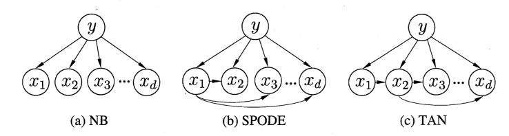
Very naturally, could the relaxation of the presumption of the independence of attribution be continued in exchange for a broader performance? Here we go back to our original problem, where the introduction of the attribute independent hypothesis is intended to address the problem of inadequate training samples due to the probability of a combination of higher levels, and the continued relaxation of this problem will fall back into the same situation again.

Bayesian Network

The introduction of the Bayesian web

Bayesian network, also known as faith network, is a tool for the development of the Internet.Directed Acyclic Graph, short DAG To define the dependency relationship between properties and to describe the joint probability distribution of attributes using the Conditional Probability Table, CPT (our example will be described as a variable-by-variant, which is virtually unlimited)

The Bayesnet is a classic probability map model.Machine learning progression and unsupervised learning: Probability mapping model

Specifically, a Beyers web.$B$ By Structure$G$ and parameters$\Theta$ Two parts. Network structure$G$ A chart with a no-ring map, each of which corresponds to one attribute, which is linked by one side if the two attributes are directly dependent. Parameters$\Theta$ Quantitatively describes this dependency if the attribute$x_i$The parent point is$\pi_i$ Parameters$\Theta$It's all there is.$P(x_i|\pi_i)$

One simple example is

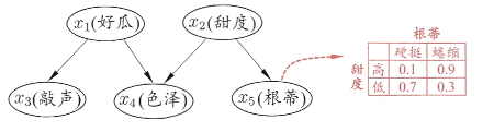
Structure of the Bayesian network

The Bayesnet has modified the ODE idea that we introduced in Park Soo Bayes, but it can be described as a broad-based PARK Soo Bayes. His structure is an effective expression of the conditions of independence between the attributes.The parent node set, the Bayesnet assumes that each property is independent of its non-descendants. Here we have to understand this sentence with There's a loopless map. Contact

So that's the definition of a joint probability distribution to $$P_B(x_1,x_2,\dots,x_d)=\prod\limits_{i=1}^dP_B(x_i\mid\pi_i)=\prod\limits_{i=1}^d\theta_{x_i|\pi_i}.$$ For the example of the habit we've been using, his combined probability is that $$P(x_1,x_2,x_3,x_4,x_5)=P(x_1)P(x_2)P(x_3\mid x_1)P(x_4\mid x_1,x_2)P(x_5\mid x_2)$$

In fact, the Bayesian network has three basic dependency structures, as follows:

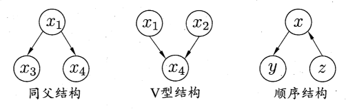
We can find a problem in the V-type structure.$x_4$ It affects his father's independence, and when the child is unknown, the two father's independence is not.

It's just a simple question of independence, and we understand the structure of the Bayesian network as sufficient.

The Beyers Network.

If the network structure is known, i.e. the dependency between attributes is known, the learning process of the Beyers network is relatively simple, and it is sufficient to estimate the probability of conditions for each node by “counting” the training sample.

In fact, we often do not know the network structure in practical applications, as in the semi-spure Beyers ODE, who is the parent node. The first task of Beyers' learning is to find the most structured "appropriate" Beyers network based on training data sets.

Query search is a common way of solving this problem. Specifically, we define a score function to assess the compatibility of the Beyeth network with training data, and then we base our search on this rating function on the best structured Beyth network. The selection of the rating functions affected the results of our last Beyers web.

Common scoring functions are usually based on informational guidelines, and we usually select the length of the code (including a description of the network). The shortest beyets, the Minimal Description Length, is the code.

Unfortunately, the best Beyers network structure is a NH from all possible cyberstructures. Hard to solve, hard to solve quickly. Two common strategies can be found to get close to it within a limited time: The first is the law of greed, the other is the method of defining structure, such as limiting the network structure to tree form.

Inference

The Beyers network is trained to answer the Query, which is through some attribute variables. The observations are used to speculate on the extraction of other attribute variables. So the process of speculating for the search of variables is called "inferment" by the observation of known variables. " (inference)

Ideally, the precise calculation of post-probability is based directly on the joint probability distribution as defined by the Beyers network, which unfortunately is difficult to extrapolate when the network has more nodes and is densely connected. We need to think about some of the more recent methods, and we're doing it now, usually using Gibbs Sampling.

You!$\mathbf{Q}={Q_1,Q_2,\ldots,Q_n}$ This means that the variables are to be asked.$\mathbf{E}={E_1,E_2,\ldots,E_k}$ For the evidence variable, the value is known to be$\mathbf{e}={e_1,e_2,\ldots,e_k}.$ Target is for post-calculation.$P(\mathbf{Q}=\mathbf{q}\mid\mathbf{E}=\mathbf{e})$of which$\mathbf{q}={q_1,q_2,\ldots,q_n}$is a group of values to be asked for variables

Gibbs sampled algorithms that produced a random piece of evidence.$\mathbf{E}=\mathbf{e}$A consistent sample.$\mathbf{q}^{0}$As an initial point, and then each step from the current sample, the next sample is produced.$t$ In subsampling, algorithms assume first$\mathbf{q}^t=\mathbf{q}^{t-1}$, then sample the non-evidence variable one by one to change the value to be taken, and the probability of sampling is based on the Beyers Network$B$, and the current value of other variables (i.e.,$\mathbf{Z}=\mathbf{z})$Calculation obtained. Assumed experience$T$Subsampling of the $\mathbf{q}$ A consistent sample is shared. $n_q$ One, which can estimate the probability of a posteriori. $$P(\mathbf{Q}=\mathbf{q}\mid\mathbf{E}=\mathbf{e})\simeq\frac{n_q}{T}.$$

In fact, this is the MCMC method of Bayesian statistics. Chain

If you want to continue to understand how the Bayesian network is being expanded into a dynamic model and how it differs from the no-turn map model, readableProbability mapping model basis: Bayesian network, the Cain Markov model and Markov airport with them。