Supervised Learning Model Evaluation: Cross-Validation, Classification Metrics, Multiclass Learning, and ROC Curves

This English version was machine-translated from the Chinese original. Technical terms may require verification.

Model assessment methodology

Errors and misalignments

The difference between the actual forecast output of the learner and the actual output of the sample is called error (error). The error of the learning device in the training set is referred to as training error or experience error; the error in the new sample is referred to as generalization error.

We would like to have a generalized learning device, but we can only try to find the one close to the smallest, what to do and what to do later.

At that point, it had to be mentioned that it was not. When the learner learns training samples too well, it is likely that some of the characteristics of the training samples themselves will be considered to be of a general nature for all potential samples, leading to a decrease in generalization performance, known as overfitting. It is contrasted with underfitting, meaning that the general nature of the training sample has not yet been learned.

An example is given below. Known columns 31, 28, 31, 30, 31, which are actually January to May days per month. To predict the next number, the simple idea is to recognize this as a month: 30 days in June. But we can also find a four-fold multiform:

$$f(n)=\frac{2}{3}n^4-\frac{25}{3}n^3+\frac{109}{3}n^2-\frac{191}{3}n+66$$

It is a precise compilation of all known values, and it is used to predict June, July, August, and it is the result of this disproportionate result of 56, 143, 346. It's typical of a match: learning a training sample too well, but not at all.

There are many factors that lead to over-adaptation, the most common of which is over-learning, which includes less general features in training samples; under-adaptation is usually caused by inadequate learning.

Unsatisfactory combinations, such as expansion of branches in decision tree learning and increased number of training wheels in neuronet learning, are better addressed. This is a much more cumbersome formulation, which is followed by a presentation of the various approaches; throughout the field of machine learning, processing is an important issue.

Traditional machine learning model

There are often multiple learning algorithms available in realistic assignments, and even using the same algorithm, different parameter configurations produce different models. Which algorithm to choose and which parameters to configure? This is the model selection problem in machine learning.

Model parameters fall into two categories. One type of automatic learning in training, such as linear regression coefficients, weight of neural network, does not require human intervention; the other category must be specified manually before the training begins, such as depth of tree models, regularity intensity, learning rate, etc., such parameters are called hyperparameters. Superparameters do not participate in the training process and can only be determined by experiment, so model selection often becomes"Pick one in a number of superparameter configurations"I don't know. The following division can be used either directly to assess the final model or to choose between configurations -- but the latter will introduce an optimistic deviation, which is what follows."Embedded Crosscheck"and"Optimistic deviation and Bootstream correction"Two sections address the issues to be addressed.

Ideally, generalization errors would be directly studied, but unfortunately they would not be available; training errors would not be used to measure generalization performance. Here's how the model is assessed.

Usually, we use experimental tests to evaluate and choose the general error of the learning device. To this end, a test set (testing set) is needed to test the learning device ' s ability to distinguish a new sample, and then the test error on the test set is applied. It's an approximation of general error. The test set should, to the extent possible, be mutually exclusive of the training package. This is from the data set. $D$ Several methods of dividing training and testing sets.

Make way.

Hold-out directly to the data set $D$ Separated into two separate collections, one for training Set $S$, the other one as test set $T$I don't know. Yes. $S$ After training the model, use it. $T$ Evaluate its test error as an estimate of the generalized error.

It needs to be noted that the classification of training and testing sets is to be as consistent as possible in the distribution of data and to avoid influencing the final outcome by introducing additional deviations, such as ensuring at least a similar proportion of the sample categories in classification missions.

In the use of the set-aside method, it is usually done several randomly, with averages obtained as a result of repeated experimental assessments.

It is common practice to train with approximately 2/3 〜4/5 samples and the remaining samples for testing.

Cross-certification

Cross certification starts with data sets $D$ Division to $k$ Close-sized mutually exclusive subsets, each of them $D_i$ As far as possible, data distribution is consistent, i.e., obtained through layered sampling.

The purpose of tiered sampling is to make each subset approximately the same category ratio as the entire data set, and to avoid a discount containing only one type of sample, leading to a serious distortion of the individual assessment. The classification tasks can be divided directly by category; the regression tasks do not have category labels, and the continuous target values are usually divided into several compartments (boxes) and then by inter-section.

Then, every time. $k-1$ The subsets are combined as a training set and the remaining subsets as a test set; this brings us together. $k$ Group training/test collection, available $k$ Training and testing and eventual return $k$ The average of each test result. Obviously, cross-validation of the results depends to a large extent on the stability and authenticity of the results. $k$ , so it is usually called k-fold cross certification.$k$ The most commonly used value is 10, i.e. 10 times cross-validation; other commonly used values are 5, 20, etc.

$k$ The extraction values represent the trade-off between deviations and deviations:$k$ The larger the set, the smaller the margin of assessment; however, the more overlapping the set, the more relevant the outcome, the greater the variance of assessment, and more models and costs to be trained.$k=10$ It is a compromise that is common in practice.$k=5$ It is more cost-effective when the amount of data is small or the model is more expensive; the amount of data can also be considered for one method, but it has a high variance (see below).

Division of data sets, similar to the set-up $k$ There are many different ways to divide the subsets. In order to reduce the differences in classification,$k$ Cross-checking usually involves the random use of different divisions. $p$ The final result is this. $p$ Minor $k$ The average of folding to cross-validation results, such as the usual 10 times 10 turns to cross-validation.

Note: Even if it's established $k$multiple cross-certification experiments - single $k$ Cross-certification produces only one average, and in the alternative, the results may vary considerably.

Repeat $p$ Another advantage of the second is the distribution of performance points: except for the average.$p\times k$ a fraction or $p$ A repeat average can be used to map the fluctuations in the assessment results, such as the calculation of standard deviations. And that's what's behind it."Cross-validation t testing"The section contains input into the hypothetical test.

Assumptions data sets $D$ Organisation $m$ A sample, if you want. $k = m$, an exception to cross-certification: leave-one-out.

Only one sample of the training set used in the retention method is less than in the initial data set, and therefore, in the vast majority of cases, the model and the use of a method of actual evaluation is retained $D$ The model of expectations that has been trained is very close and the results are often considered to be more accurate.

However, there are two obvious shortcomings in retaining one. One is to calculate the cost: training is required when the data set is larger $m$ A model that calculates costs that may not be affordable (e.g., a data set containing 1 million samples requires training 1 million models), which is not yet accounted for by algorithms. The second is the fact that the difference is high, which is counterintuitive: while it is almost neutral, each test set has only one sample, the single result is highly volatile, and each training set is highly overlapping.$m$ The results are highly correlated, and the average difference is not equal to the discount. $k$ Collapse small validation. Therefore, leaving a method to estimate deviations on small samples is valuable, but does not add value to unstable algorithms (e.g. decision tree, k neighbourhood) or large data sets.

Cross-validation for model selection: nested cross-validation

The cross-certification described above is based on the assumption that the final model will be assessed on a fixed division. However, the actual process is often preceded by cross-validation of over-parameters or algorithms - one of the highest scores in a number of candidate profiles. Once this is done, the results of the assessment carry an optimistic bias: you have chosen the best of the many candidates, its scores are naturally optimistic, and the same data is used to evaluate it.

To obtain a generalized error estimate of the transposed model, it is necessary to use embedded cross-validation: the outer layer divides the data into several discounts, leaving them to be assessed; and the inner layer performs another cross-validation of the training component at each discount to select the hyperparameter. Internal responsibility."Choose"External responsibility"Commentary"The data used for the two layers are completely isolated, and what is available is an unbiased error estimate of the reference model.

Embedded cross-certification costs a lot more (the outer layer runs a full internal duct at each turn). Thus, when models are only used to make final predictions and do not seek externally declared impartial error estimates, there is usually no need to embed them: the direct inner layer cross-checks the selected parameters and then the full data is trained. The more common practice in in-depth learning is the fixed training/certification/testing division (see later)."Evaluation of in-depth learning models"The essence is to simplify the embedded structure into a single layer.

Non-independent data: grouping and time series cross-checking

All of the previous classifications implied the assumption that the samples were independent of each other and could be distributed randomly. When this assumption does not work, random classification leaks information - samples from the same source are distributed into both training and testing sets, and the results are not high. Two common types of situations:

• Group Data: Multiple samples produced by the same testee, the same equipment or the same experiment. In this case, the entire group should be drawn to the same side, ensuring that the same sample is either in the training set or in the test set, i.e. cross-checking in groups (group k-fold).
• Time series: Samples are sorted over time and future information cannot be used to predict the past. In this case, a time-series split should be used (above) $t$ A moment of training.$t+1$ Time test) e.g. rolling predictions without random disruption - otherwise equivalent"Look at the future."。

Bootstrap

In addition to the first two, there is an assessment method that is less useful. Organisation $m$ Data sets for each sample $D$, generate a data set for its sampling'$：每次随机从 $D$ 中挑一个样本，拷贝放入 $D'$，再把它放回 $D$，使它在下次采样时仍可能被采到；重复 $Mm-hmm.

Some 36.8% of the initial data concentration through self-help sampling would not appear in the sample set $D'$ 里。于是可以用 $D'$ 作为训练集，用未出现在 $D'$ 中的样本作为测试集。这样，实际评估的模型与期望评估的模型都用了 $m. A training sample of US$ 1/3 of the total data was tested and did not appear in the training concentration. The results of such tests are also referred to as off-pack estimates (out-of-bag estimate).

The self-help approach is useful when the data sets are small and it is difficult to effectively divide the training/test sets; in addition, it can produce many different sets of training from the initial data collection, which can greatly benefit such methods as integrated learning.

However, the data set generated by the self-help approach alters the distribution of the initial data set and introduces estimates deviations. As a result, leave and cross-certification methods are more common when the initial amount of data is sufficient.

Here, only the self-help method is used as a data disaggregation and assessment strategy; its more common identity is the statistical extrapolation tool - the equations, deviations and confidence compartments in which a re-sampling of any statistical amount is estimated, as well as the Jackknife, Subsampling method with its own ethnic group, as described in more detail.The computational revolution of statistical extrapolations: details of Jackknife, Bootstream and Subsampling》。

Optimistic deviation and Bootstream correction

It's all left in front, cross-checked."Error on test set"It's been separated from training. But there's a more modest assessment benchmark to be vigilant:The error on the training set.As a model of good and bad indicators. This error is called apparent error, and it is called re-adaptation error:"For yourself."Naturally low. The difference between a watch error and a true error is an optimism:

$\text{optimism}=\mathbb{E}\big[\text{Specific Error}-\text{True Error}\big]>0$$

Optimistic deviations arise from over-alignment: the stronger the training, the better the appearance, the less the general error, the less the optimism. The ideal thing is to take it out and add it back.Correction Error $=$ Watch error $+$ Optimistic deviationI don't know. The idea behind the Bootstream rectification (Efron 1983) is to calculate the optimism bias itself by replicating it:

1. In Raw Data $D$ We're going to have a model. $A$；
2. There's a Bootstream sample put back to take. $D^}$，在 $D^{}Adjust Rework ModelReplay all modelling steps: Select the features, toggle the parameters at $D^}$ 内重做，否则偏差被低估），得到 $\hat{\theta}^{}$；
3. Yes. $D^{*}$ Calculate the error of this model (playing)"Training error") In original $D$ Add its error."Test Error"）；
4. The difference between the two is $mathrm{Err} (D,hat{\theta}})-\mathrm{Err}(D^{This is an optimistic deviation estimate.
5. Repeat $B$ (General) $B\ge 200$Average $\hat{O}$, the correction error is $A+\hat{O}$。

Intuitively, every Bootstream sample is one of the original data."Supersync": Model in $D^{*}$ The error on it."More than proposed"In original $D$ The error on it."It's done."The difference between the two is simulated."- No match."And that is the optimism bias itself. That's why raw data can be used here."Test Set"- Every bootstream sample is generated from it.

Optimistic correction also has a well-known variant, which weighs the average of appearance errors and outlier errors:

$$\hat{\mathrm{Err}}_{.632}=0.368\cdot A+0.632\cdot\varepsilon^{(B)}$$

of which $\varepsilon^{(B)}$ That's the old story."Bootstrap"A section of the error (leave-one-out Bootstream) measured in OOB samples. Watch error $A$ It's too optimistic.$\varepsilon^{(B)}$ It's too pessimistic -- each test point appears on average only in about 63.2% of the Bootstream sample, which is equivalent to only about 63.2% of data training; 0.632 This weight comes from $1-e^{-1}$I don't know. Use 632+ (Efron) when serious & Tibshirani (1997) $\varepsilon^{(B)}$ The weight.

Simple comparison with embedded cross-validation: Both are modified by the same type of deviation, which also requires the repositioning of all modelling steps within the re-sampling, but with different pathways:

	Embedded Crosscheck	Bootstream Optimistic Correction
Source of deviation	Use the same data for + assessment and select the best candidate	Watch errors test themselves on training data.
Method of amendment	Exterior fold assessment, internal folding, data segregation	Re-sampling estimates for optimistic deviations.
Do you need to draw out the test? Set	Required (outside fold, test set)	No need. Original data is also tested. Set
Cost	Every turn of the outer layer, the inner layer, it's expensive.	Yes. $B\ge 200$ Secondary complete modelling
Typical scene	You have to make a statement about errors and make model choices.	Few samples and a reluctance to waste data (e.g. clinical prediction models)

This section discusses the results of the assessment."Offset", relative to"Difference"See section below for questions.

Differences and differences in assessment results

Various assessment methods were discussed in previous sections, but were not systematically discussed."Assessment itself"The statistical nature. The number of the evaluation method output is also a function of the data, with the same deviations and deviations, and the deviations-square structures of different methods vary considerably. Many of the seemingly contradictory conclusions in practice are in fact a mixture of these two errors.

Training cluster assessment and cross-validation station at two diagonal sides of the deviation-square plane：

	Offset	Difference
Training set (watch) evaluation	Large: Optimistic bias, fixed direction low	Small: Full data, no randomity
Leave / Cross-check	Small: Approximate	Large: Test collection is only part of the set and is randomly divided

This explains a common phenomenon: one high-capacity model (e.g., XGBoost) is much better than the others in the training set, but it is not different when cross-checked. The former is the dominant bias."How many questions do you have?"; the latter is the factor-driven -- cross-validation is"How much can it be?"And none of the scores of the models in the small sample can be seen in the same noise.

The difference in assessment estimates can be broken down into layers., each layer can only be pressed by the corresponding means:

1. Data itself: The data are only a sample of the total, and this part of the noise is not available and can only be increased by data;
2. Randomity of the folding: a division, with different models and results, with repeated cross-checking;
3. Randomity of model formulationXGBoost subsampleAnd random forest sampling makes each one random; a small sample."Almost got a model."The model itself is highly volatile and relies on fixed seeds, multiple proposed consolidation of averages, and reinforcement of regularity;
4. Estimation of indicators on hyper-small test set Bad: This layer is the deadliest in unbalanced data. The ratio estimate is about $p(1-p)/n$The denominator is actually...Number of sample categories– Assuming a few categories of 30 and a five-percent discount, there are only about six regular cases per fold test set. F1, AUC takes the value on such a set of tests:"Jump"In the case of single-dependent fraction fluctuations of more than ± 0.1, the real difference between models (perhaps only 0.02 ~ 0.05) is completely submerged.

There is also a hidden source of differences: selection.'s curse）I don't know. The highest score in a number of candidate models or hyperparameter configurations is equal to the maximum of a bunch of noise estimations, and the maximum value expectations will be one quarter higher than the true best (the maximum of the independent peer estimate is about) $\sigma\sqrt{2\ln m}$，$m$ Is the candidate? So it's particularly dangerous to pick models in training packages. That's the reverse selection of the most optimistic bias model; even if cross-checked, if the same data were used, the best-configured fraction would have been the selection deviation, as mentioned above."Embedded Crosscheck"A section to strip off something.

What level is the double cross-check pressure? Repeat $p$ The second time, the second, the second, the second, the second, the second, the second, the second, the second, the second, the second, the second, the second, the second, the second, the second, the second, the second, the second, the second, the second, the second, the second, the second, the second, the second, the second, the second, the second, and the second, the second, the second.$p\times k$ The score is not independent and the number of valid samples is much smaller than $p\times k$The difference doesn't work. $1/\sqrt{pk}$I don't know. To compare two models, all models should be usedSame group of foldsMatching - common fluctuations between folds are divided and the difference is much smaller than the split assessment, which is also"Cross-validation t testing"The raison d ' être of the section.

Practical list of variations：

Difference Source	Response
Data itself	Only add data.
Collapse	Repeat layer cross-validation, report average ± standard deviation
Model for randomity	Fixed seeds, multiple proposed consolidation of averages, enhanced regularization
Indicator estimate	Replace the threshold category with continuous indicators (log-loss, Brier); look at PR-AUC under imbalance instead of Accuracy/ROC-AUC
Participation/option	Embedded cross-check, put"Choose"and"Commentary"Data segregation

Note: The instability of log-loss and PR-AUC in small samples, when carefully cross-checked, may result in the continued reduction of the samples and significant variations in estimates. It is generally recommended that Bootstream be considered at this time to control the difference.

Summarized in one sentence: The training cluster assessment (low variance, high deviation) and cross-validation (low deviation, high variance) are measured in different amounts and read in combination"Paradox."Conclusions. When you evaluate a model, you put it first."What do I have to measure, what's the deviation and what's the difference?"Think clearly - the deviation can be corrected (see previous section) and the margin can only be reduced by experimental design.

Evaluation of in-depth learning models

In in-depth learning, we divide the original data set directly into three parts:

• Training Set
• Authentication Set
• Test Set

The training set is used for model learning, the validation set is used for hyperparametric regulation, and the test set is used to measure the generalization performance of the model and to evaluate its effects.

The combination of validation and testing should not be divided into two, otherwise there may be oversatisfaction (which in fact results in a leak of information); what should be avoided is the centralized selection of test sets from training.

The basic workflows are: training package model training set validation set ultraparameter adjustment final model set test set final performance assessment.

From the point of view of embedded cross-certification, this three-part division is actually its degradation form: certification cluster carrying"Internal Selection"The role, the test set."Outer level assessment"It's a role, but it's only done once on each floor. It's not really embedded because the in-depth learning training is too expensive -- a model is expensive enough to run the whole inner circle in every turn, like a traditional machine."Purgatory"The number of times is limited, with fixed threes being a pragmatic option subject to cost constraints. If the amount of data allows and requires a declaration of impartial error estimates, it can still be returned to the previous text. ]"Embedded Crosscheck"The embedded approach of the section.

Control of percentages:

• Small samples (millions of scale): 60% training set, 20% validation set, 20% testing Set
• Large samples (tens of thousands of scale): Sufficient number of validation and test sets, e.g. fixed 100,000 each
• Fewer over-parameters: appropriately reduced validation collections, with samples handed over to training Set
• Very little data: traditional ML methods, such as cross-validation (extraordinary error estimates to be declared after reference, cross-validation with embedded kits, see above)

Multimodel comparison test

A direct comparison of the size of performance measures may not be a good judgement model:

First of all, we want to compare generic performance, while the experimental assessment produces performance on the test set, which is not necessarily consistent;

Second, the performance on the test set is highly relevant to the choice of the test set itself. Test assemblies of different sizes have different results; even if they are the same size, they contain different test samples and the results vary;

Thirdly, many machine learning algorithms themselves are somewhat random, and even if they run multiple times on the same test set with the same parameters, the results may be different.

So, is there an appropriate way to compare the performance of the learning machine?

Statistical hypothesis tests (hypothesis test) provide an important basis for learning machine performance comparisons. On the basis of the hypothetical test results, we can assume that if a learning device A is better than B on the test set, then the generality of A is really better statistically than B, and how sure it is. (The first two points were circumvented by multiple test sets and the third was addressed by statistical hypothetical tests.

Two basic hypothetical tests are presented below, followed by several commonly used machine learning comparison methods. For ease of discussion, this section defaults to measure performance by error rate.

Assumptions test

Multiple experiments provide a basis for the use of statistical hypothetical tests by obtaining multiple, rather than only one, error-rate observations.

Hypothetically, the probability of a learning device making a mistake in each sample is... $p$I don't know. In a training and testing, we know the size of the test set and the number of errors, so we can use the error rate. $p$ A hypothetical test to determine whether the learning device is at a given value (the error rate assumption test for a training and test).

Sometimes we do it more than once, but we get multiple test error rates through multiple repetitions or cross-checks, at which point the average error rate can be estimated and hypothetically tested (multiple error rates, essentially average t tests).

Cross-validation t testing

More often, we want to assess the differences in performance between multiple learning devices, using cross-validation t tests, i.e. data t tests: multiple learning devices give results for the same training and testing, and the data are paired.

It should be recalled that this test is not strictly established in theory: t Tests assume that groups of observations are independent of each other, but cross-validation of training sets overlaps, inter-calibration results are not independent, and standard cross-validation t tests underestimate differences and can easily overestimate visibility. Amendment practices such as 5x2 cross-validation (Dietterich 1998), which are commonly used in practice, are mitigated by the random split of data, with one training on a rotational basis, one test (one double in a repeat) and five repetitions of 5 logarithms, which are used to construct statistics similar to the t-distribution of the scores, and reduce reliance on overlapping training sets.

McNemar Test

In the case of two algorithms, two classes, one can list the correct or incorrect combination of tables for each algorithm; if it is assumed that the performance of the two classification algorithms is not different, it can be handled with a calibration.

Friedman test and Nemenyi follow-up

It is used to compare the overall performance of multiple algorithms at a time that is easier than cross-validation of t tests, which do not require two or two tests.

Performance measures for classification models

The experimental design methods for estimating learning instrument performance were described earlier, and performance measurement indicators are now required. Performance measures reflect mission requirements.

When comparing the capabilities of different models, different performance measures are used, often with different judgments. This means that models are relative: what models are good depends not only on algorithms and data but also on mission needs.

In the classification tasks, performance measures study the differences between real and projected categories.

Error rate and accuracy rate

Naturally, the following two indicators can be given to reflect the good and bad model:

• The error rate is the percentage of the number of samples that were classified wrong to the total number of samples
• Accuracy rate is the proportion of the number of correctly classified samples to the total number of samples

It is easy to see the sum of both as 1. However, such indicators are insufficient and require further study.

Measurement based on a matrix

The error and accuracy rates are common but do not meet all mission requirements. For example, we are often concerned that “how many of the targets are really to be selected”, which cannot be measured by the preceding indicators and therefore requires additional indicators.

According to Real Class Tags $D$ and predictive type labels $R$ Scoping of samples is available $k\times k$ . . . . . . . . . . . . . . . . . . . . . . $N(i,j)$, where the location elements are $n_{ij}$I don't know. The following is an example of a two-category confusion matrix.

Category Identification Rate

Catalogue $M$ On categories $c_i$ Rate of approval defined as predicted $c_i$ The proportion of the sample that is projected to be correct is:

$$\mathrm{prec}i=\frac{n{ii}}{m_i}$$

of which $m_i$ It's a sorter. $M$ Projected $c_i$ Number of samples for class.

The overall accuracy rate of the taxonomy is the correct sample of all projections:

$$\mathrm{Accuracy}=\frac{1}{n}\sum_{i=1}^k n_{ii}$$

This is the accuracy rate of the preceding definition. It needs to be noted that accuracy is not the same indicator as precision.

Recall

Full-scale measures should have been classified $c_i$ The proportion of samples correctly identified by the model:

$$\mathrm{recall}i=\frac{n{ii}}{n_i}$$

of which $n_i$ Is the real category is $c_i$ the number of samples.

F1

Classifiers usually face a trade-off between the rate of approval and the rate of full coverage, and ideally we want both to be as high as possible.

Each category F-measure tries to balance the accuracy rate and the overall rate. It's a category. $c_i$ reconciliation between precision and recall:

$$F_i=\frac{2}{\frac{1}{\mathrm{prec}_i}+\frac{1}{\mathrm{recall}_i}}=\frac{2\cdot\mathrm{prec}_i\cdot\mathrm{recall}_i}{\mathrm{prec}_i+\mathrm{recall}i}=\frac{2n{ii}}{n_i+m_i}$$

$F_i$ The higher the value, the better the sorter.

Catalogue $M$ The overall F-measure is the average of the various F-measure categories:

$$F=\frac{1}{k}\sum_{i=1}^{k}F_i$$

Confusion matrix on classification issues

Among the issues of the second classification, the sample can be divided into four scenarios, based on a combination of the true and projected categories of the sample, namely, true form, false form, genuine offence, and false form.

TP + FP + TN + FN = total number of samples. The confusion matrix for classification results is as follows:

The truth.	Projected results: positive examples	Projected results: reverse examples
Positive	TP (real example)	FN
Reverse	F.P.	TN

Error and accuracy (II classification)

The proportion of error predictions, as described in the previous section “Errority and accuracy”:

$$\mathrm{Error~Rate}=\frac{\mathrm{FP}+\mathrm{FN}}{n}$$

The correct projection is the accuracy rate:

$$\mathrm{Accuracy}=\frac{\mathrm{TP}+\mathrm{TN}}{n}$$

Rate of approval and full coverage

Classification II is an exception to the preceding category of indicators. Positive and negative categories were identified as target categories, with rates of approval:

$$\mathrm{prec}{P}=\frac{\mathrm{TP}}{\mathrm{TP}+\mathrm{FP}}=\frac{\mathrm{TP}}{m_1};\quad\mathrm{prec}{N}=\frac{\mathrm{TN}}{\mathrm{TN}+\mathrm{FN}}=\frac{\mathrm{TN}}{m_2}$$

When the trade-off between the rate of approval and the rate of fullness is usually discussed, the default focus is on the positive category. The success rate requires that the number of cases selected be as accurate as possible, i.e., that there be fewer choices; and that there be as many cases of actual cases as possible, i.e., that there be more options.

Sensitivity and specificity

Sensitivity is the positive rate, while specificity is the negative rate:

$$\mathrm{TPR}=\mathrm{recall}_P=\frac{\mathrm{TP}}{\mathrm{TP}+\mathrm{FN}}=\frac{\mathrm{TP}}{n_1}$$

$$\mathrm{TNR}=\text{specificity}=\mathrm{recall}_N=\frac{\mathrm{TN}}{\mathrm{FP}+\mathrm{TN}}=\frac{\mathrm{TN}}{n_2}$$

Fake and positive.

Sensitivity and specificity are different from 1.

$$\mathrm{FNR}=\frac{\mathrm{FN}}{\mathrm{TP}+\mathrm{FN}}=\frac{\mathrm{FN}}{n_1}=1-\text{sensitivity}$$

$$\mathrm{FPR}=\frac{\mathrm{FP}}{\mathrm{FP}+\mathrm{TN}}=\frac{\mathrm{FP}}{n_2}=1-\text{specificity}$$

Integrated measurement methods

This is still based on the confusion matrix of the second category. Where there is a category imbalance, confusion of absolute numbers in the matrix may not be very useful, so the following approach is introduced, which is intended to give a more integrated model performance assessment of classifications. For the treatment of imbalances, seeUneven practice processing of samples。

PR Curve

Defines the positive rate $P$ and full coverage $R$：

$$\begin{aligned}P&=\frac{TP}{TP+FP},\\R&=\frac{TP}{TP+FN}.\end{aligned}$$

In many cases, samples can be sequenced according to the results predicted by the learner, and the first is considered the most likely, and the last is the most unlikely. Let the classification threshold move from high to low and each threshold gets a set $P$、$R$I don't know. A P-R curve is obtained using a cross-axis and a cross-axis check.

If the P-R curve of one learner is completely enclosed by the curve of another learner, it can be asserted that the latter perform better than the former.

The area below the P-R curve is normally recorded as PR-AUC, which aggregates the entire curve into a value.

F Measure

Complete coverage is rare, and it is normal to cross the curve. If you need to compare a single work point below a classification threshold, you can measure using F1. Follow the symbol of the previous "F1" section:

$$F_1=\frac{2\times P\times R}{P+R}=\frac{2\times TP}{\text{样例总数}+TP-TN}$$

It is the reconciliation of the rate of approval with the average of the rate of full coverage.

In some applications, yes. $P$、$R$ There are different degrees of emphasis, so there are also broad F1 measures called $F_\beta$：

$$F_{\beta}=\frac{(1+\beta^{2})\times P\times R}{(\beta^{2}\times P)+R}$$

$\beta$ The importance of the two: $\beta>1$ 时更看重查全率，$0<\beta<The rate of rechecking is higher at $1.00. It is essentially weighted and average.

For multi-classification issues, they are often translated into multiple two-class questions; at this time there are multiple confusing matrices that can calculate the averages of TP, FP, TN, FN and then the F1 measures.

ROC and AUC

Many learners produce a real or probabilistic projection for the test sample, which is compared with the classification threshold (threshold) and is rated more than the threshold as positive or otherwise negative.

The probabilities of this real or probabilistic projection directly determine the generalization of the learning instrument.

Thus, the quality of the ranking of projections reflects the broadness of the learning machine ' s expectations at different thresholds, and the ROC curve is a powerful tool for studying the generality of performance from this perspective.

Similar to the PR curve, the sample is sorted into a sample based on the projection results, and the sample is projected as a regular case by case, each time a value of two critical quantities is calculated, using them as cross- and vertical coordinates.

The vertical axis of the ROC curve is the true normal rate (TPR), and the horizontal axis is the false normal rate (False Popular Rate, FPR):

$$\begin{aligned}\text{TPR}&=\frac{TP}{TP+FN}\\\text{FPR}&=\frac{FP}{TN+FP}\end{aligned}$$

When comparing learners, similar to the P-R figure, if the ROC curve of one learner is completely enclosed by the curve of another learner, the latter can be asserted to perform better than the former;

If two ROC curves intersect, it is difficult to generally assert who is the best and who is the worst. At this point in time, the more reasonable criterion is the size of the comparative curve, namely, AUC (Area Under ROC Curve):

$$\mathrm{AUC}=\frac{1}{2}\sum_{i=1}^{m-1}(x_{i+1}-x_{i})\cdot(y_{i}+y_{i+1})$$

In general, AUC explains as follows:

• AUC = 0.5: Indicates that the model does not have the capability to classify, which is equivalent to random speculation.
• 0.5 < AUC < 0.7: Indicates that the model has some sort of classification capability, but has a general effect.
• 0.7 ≤ AUC < 0.9: Indicates that the model has a better classification capability.
• AUC ≥ 0.9: indicates that the model has a very good classification capability.

ROC-AUC is the most commonly used disaggregated performance assessment indicator, which is practical and not sensitive to uneven categories.

Indicator selection in an unbalanced scenario

When there is a serious imbalance in the distribution of categories, each of the above indicators has its own blind regions, and the main points of trade-off in practice are as follows:

Indicators	Answer what?	When would it be misleading to be unbalanced?
Accuracy	What's the overall forecast?	It's very rare to be in most categories."Push!"
AUROC	Is the whole rule ahead of the negative?	The negatives may look good when they're too many, but there's still a lot of misreporting.
PR Curve / AUPRC	How many of the positive samples are real and how the recall losses change?	Baseline changes with prevalence and cross-data set comparisons need to be reported a priori
Balanced Accuracy	Average of categories	It doesn't reflect probability calibration, it doesn't reflect miscalculated costs.
MCC	Whether the matrix is balanced or not	Still unable to replace per-class indicators and threshold analysis
Macro-F1	Is tail also visible?	Sensitivity to thresholds and subcategory sample numbers
Brier / ECE	Is the probability output credible?	A poorly sequenced model may not be available even after calibration.

The PR curve tends to reflect real pressure more than ROC: ROC takes in a lot of real negatives, and many models appear."Not bad.", and PR space is more directly exposed to misrepresentation of costs. However, as the PR baseline is bound by Prevalence, AURPC is required to report both positive ratios across data sets.

In multi-classical missions, Micro indicators are naturally close to the overall performance of head class and can easily hide problems. To judge whether tail class is really improved, at least the macro indicator, per-class indicator, confusion matrix and head/media/tail layer results are given simultaneously. I'll see you in a more systematic way.Uneven practice processing of samples。

Multi-category learning

For the issue of multi-classifications, there has been no systematic presentation of how to construct multi-classification models, and only a brief reference to multiple-style Logit is made in Logistic returns. Here are some of the most common ideas:Dismantling the issue of multi-classification into more than one category。

One vs. One $N$ Two pairs of disaggregated data sets. $N(N-1)/2$ Each sorter is trained separately. New samples are submitted to all taxonomyrs when forecasting. $N(N-1)/2$ The results are classified in two categories and the final results are obtained by vote.

One vs. Rest (OvR) uses one type of sample as a positive example each time, and all the rest of the categories as an example. $N$ A sorter. If only one classifier is projected as a positive class at the time of the test, the corresponding category is used as the final result; if more than one classifier is projected as a positive class, the forecast confidence of each classifier is compared and the largest category is used as the classification result.

Many vs. Many (MvM) treats several categories as positive and several others as inverse, and Ovo and OvR are its exceptions. The most commonly used technique to construct a positive and negative classification is the correction output code (Error Corracting Output Code, known as ECOC), which has some ability to correct errors. Two steps:

• Encoding: Right $N$ Multiple classification of individual categories, each of which classifies a part of the category as positive and a part as inverse, resulting in a two-category training set; $M$ A training set. $M$ A sorter.
• Decoding:$M$ Each taxonomy predicts the test samples, and the predict mark consists of a code that compares with the respective code for each category and returns the lowest distance category as the final projection.

A common coding matrix (coding matrix) is:

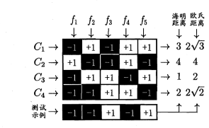
N.B.: Both OvR and MvM, split sub-categories may be re-incorporated into category imbalances in a way that can be addressedUneven practice processing of samples。

It's a classic general framework, but most of the mainstream libraries are now gone.Primary categoryRoutes, which do not really train several independent classification models:

• The tree model (decision tree, random forest) is directly divided by several types of impurity, with natural multiple classifications;
• GBDT (XGBoost) multi:softprobLightGBM multiclass) Train one tree per cycle for each type, combined optimized with softmax cross-cream, one integrated direct output $K$ Type probability;
• Softmax returns, single models,$K$ Group weights;
• Neurological network loss with softmax output layer plus cross-radon.

Still retaining split lines at the nuclear SVM (libsvm internal OVO) and sklearn OneVsRest/OneVsOne Packaging. The split perspective, however, remains important in multi-classification assessments - the expansion of ROC in the following section is carried out by category OvR.

Performance assessment under multiple categories

The confusion matrix, accuracy rate, category-by-category indicators, PR/ROC could be used for the issue of multiple classifications, but all needed to be expanded appropriately. The following is a description of how this is calculated and how it looks under the multiple categories.

Confusion MatrixYes. $K\times K$ : No. $i$ Line $j$ Column is the real category as $i$projected $j$ The number of samples is the correct number for each category. When you look, focus.High value position on non-diverse line- That's the most confusing category.

** Accuracy** is the sum of the diagonal elements divided by the total number of samples. Blind zones are dominated by the majority when there is an imbalance in categories, and a few complete errors may also be very high.

Category / Recall / F1: Each category rotates as"Normal"for the remaining categories"Inverse"(OvR perspective) Each category has a set of precision, recall and F1. This is the basis for determining whether tail class is taken care of.

Macro, micro and weighted averages— Three ways of grouping indicators into one number of hours:

• Macro• Directly average the various types of indicators, with equal rights for each category, and more sensitive to the few sample categories;
• Micro-average (Micro)(a) The combination of all categories of statistics into a single table, which is equal to the weighting of samples, and the natural proximity of multiple groups of samples (Micro-F1 for multiple classifications is exactly the same as Accuracy);
• Weighted: weighting of indicators by category by sample, between (sklearn) average='weighted'）。

Micro indicators in multi-classical long-term assignments are usually beautiful, but are often only good for the head category; depending on whether the tail category is actually improved, they need to be reported together with the Macro indicators, the category-by-category indicators and the confusing matrix.

ROC / AUC: Expands by class with a ROC curve for each class, and AUC takes macro or weighted average by sample. When categories are uneven, the PPR curve after OvR tends to reflect the actual performance of a few categories better than ROC, depending on the above"Indicator selection in an unbalanced scenario"Section.

Return Model Performance Measure

Back to the basics of model measurements

The performance measure for the regression mission is the projection. $f(\boldsymbol{x}_i)$ And real value $y_i$ Gaps, data sets $D$ Organisation $m$ A sample. Common indicators are broadly divided into three categories: one looking at absolute errors and the other $y$ The equation, the numerical intuitive, but different punishments for different samples; one looking at the interpretation or percentage relative to the baseline, eliminating the matrix and facilitating horizontal comparisons; and one specifically designed for high-level, right-wing data. This is presented below by cluster.

MSE, MAE and RMSE

The three indicators are the most basic error measures to be returned, along the same lines: the number of errors per sample is aggregated to indicate how much the model as a whole is different. The difference is in the way of aggregation.

$$E(f;D)=\frac{1}{m}\sum_{i=1}^{m}\left(f\left(\boldsymbol{x}{i}\right)-y{i}\right)^{2}$$

Average error (MSE) equals the error squared to the L2 measure. The squares magnify larger errors, so if there are a few samples with large deviations, MSEs will be significantly elevated and sensitive to anomalies; in turn, large errors in training will be modified. Square also allows the function to be guided and visible and is the most convenient loss function to optimize. MSE unit needs attention. $y$ , the value itself is not intuitive.

$$\mathrm{MAE}=\frac{1}{m}\sum_{i=1}^{m}\left|f(\boldsymbol{x}_i)-y_i\right|$$

The average absolute error (MAE) takes the average of the absolute value of the error, which is the L1 measure, and the error of each sample is treated as right. Individual abnormalities can only add a little bit to the whole value, and are therefore better; the disadvantage is that they do not highlight large errors, and that as a loss function they are unguided, the gradient is constant, and the contraction is slightly lower than MSE. Its units and $y$ Consistently, the average difference in reporting is the most intuitive.

$$\mathrm{RMSE}=\sqrt{\frac{1}{m}\sum_{i=1}^{m}\left(f(\boldsymbol{x}_i)-y_i\right)^{2}}$$

The RMSE is the MSE root, which is the unit from $y^2$ Pull back. $y$Read as if, on average, the error is about as large as it is a form commonly used in the report. Its punitive character is exactly the same as MSE, as sensitive to abnormal values. Where there is a significant gap between the MAE and RMSE values of a model, it is usually suggested that a small number of large discrete points are mixed in the error.

There are two more extreme variants in the same category: Max Error takes the maximum value for all samples, reflecting the worst-case scenario, and is suitable to judge whether the model is stable in key samples; the median for the median absolute error (MedAE) is better than MAE, and is almost unaffected by extreme anomalies.

R2 and adjustment R2

$$R^2=1-\frac{\sum_{i=1}^{m}\left(f(\boldsymbol{x}i)-y_i\right)^{2}}{\sum{i=1}^{m}\left(y_i-\bar{y}\right)^{2}}$$

of which $\bar{y}$ is the average of the real value. The idea of determining the coefficient (R2) is to find one of the simplest opponents: to learn nothing, to set the projections in average. $\bar{y}$I don't know. The denominator is the sum of the error squares of the baseline, and the molecules are the sum of the error squares of the model, and the contrast of the two is that the R2 measure is how much of the error of the model is less than the baseline or how much of the difference is explained. equals 1 to perfect alignment, equals 0 to a direct projection average, which is negative when compared to the baseline. It does not have a schematic framework, allows comparisons between different missions, and is almost necessary in returns reports. The disadvantage is that it does not reflect absolute error sizes: a task with a high target value, with a much worse projection of R2 and a higher number of R2 features on the training set.

$$\bar{R}^2=1-\left(1-R^2\right)\frac{m-1}{m-p-1}$$

of which $p$ is the number of features. Adjustments to the decision factor (Adjusted R2) are revised on the R2 basis by the number of features: for each additional feature, the adjusted value will decline unless it really explains the additional deviation. Therefore, when comparing models with different number of characteristics, or selecting features, the adjusted R2 should be seen to avoid using stack features to draw up values.

MAPE and SMART

$$\mathrm{MAPE}=\frac{1}{m}\sum_{i=1}^{m}\left|\frac{y_i-f(\boldsymbol{x}_i)}{y_i}\right|\times 100%$$

The average absolute percentage error (MAPE) divided the error per sample by the real value and obtained the average. The idea is that on average it is wrong, that the report gives non-technical readers the most visual and naturally eliminates the matrix and allows comparison of tasks with completely different target scales. There are two disadvantages: when the real value is close to 0, the error is divided by a small number that explodes or is not even defined; and the same absolute deviation, with the punishment for the small sample being heavier, overvaluation and underestimation being asymmetrical.

$$\mathrm{SMAPE}=\frac{1}{m}\sum_{i=1}^{m}\frac{\left|f(\boldsymbol{x}_i)-y_i\right|}{\left(\left|y_i\right|+\left|f(\boldsymbol{x}_i)\right|\right)/2}\times 100%$$

The symmetrical absolute percentage error (SMAPE) swapped the denominator to the average of real and projected values, which alleviated the problem of the real value in the MAPE when it exploded close to 0, and raised some symmetrical and undervalued penalties. The price is not as good as MAPE's intuitiveness, and the projection is still unstable when it comes to 0, and needs to be noted when it is used.

RMSLE

$$\mathrm{RMSLE}=\sqrt{\frac{1}{m}\sum_{i=1}^{m}\left(\log\left(f(\boldsymbol{x}_i)+1\right)-\log\left(y_i+1\right)\right)^{2}}$$

The average root logarithmic error (RMSLE) starts with a logarithmic of the projection and the real value (plus 1 to allow 0 to get a logarithmic) and then calculates RMSE on the scale after the logarithm. The idea is to replace absolute error with relative error: The absolute error allowed when the target value is large is also significant and the target value hour is more demanding. It is therefore appropriate for the task of several orders of magnitude, such as house prices, sales and so forth, where there are significant differences in the level of the target. For the same goal, underestimation is more severe than overestimation, and models are pushed to Ninkendo and not missing; projections are required to be non-negative.