Probabilistic Graphical Models: From Bayesian Networks to LDA

Introduction: Probability structure expressed in graphics

When hundreds of variables are reached, the direct modelling of the combined probability distribution $P(X_1, X_2, \dots, X_n)$ Often not feasible: the number of parameters increases exponentially with the number of variables.Probability chart model(Probabilistic Graphial Models, PGM) uses graphics to express the structure of the variables, quantify the intensity of dependence with probabilities, and thus disassembly the joint distribution of the high dimensions into a local, interpretable part.

If you want to move from a condition-based assumption in a classification mission to the subject, you can recall thatMachine Learning Introduction and Monitoring Learning: The Bayesian CatalogueI'm sorry. The PARK Soo-Bayes and PARK Soo-Bayes to the Bayesian network are the same path that gradually relaxes the assumption of identity independence.

This paper places four representative models in the same framework:

Model	Figure structure	Main Process Objects	Expression of condition independence
Bayesian Network (BN)	A-DAG-DAG-DAG-DIG-DIG-DIG-DIG-DIG-DIG-DIG-DIG-DIG-DIG-DIG-DIG-DIG-DIG-DIG-DIG-DIG-DIG-DIG-DIG-DIG-DIG-DIG-DIG-DIG-DIG-DIG-DIG-DIG-DIG-DIG-DIG-DIG-DIG-DIG-DIG-DIG-DIG-DIG-DIG-D-D-DIG-D-D-DIG-D-D-D-D-D-D-D-D-D-D-D-D-D-D-D-D-D-D-D-D-D-D-D-D-D-D-D-D-D-D-D-D-D-D-D-D-D-D-D-D-D-D-D-D-D-D-D-D-D-D-D-D-D-D-D-D	Static variable depends on	Local independence after the given parent node
The Cain Markov Model (HMM)	A directional map over time	Sequence and Hiding	Current status depends only on the previous status
Markov Airport with MRF	No Flow	Symmetrical spatial or neighbourhood relationships	Conditional independence of the figure after separation
Potential Dilekre Allocation (LDA)	Prospective Generate with Plate Figure	Document and potential theme	When assigned to the given theme, the word is only based on the corresponding theme

The four share the idea of “the structure of the map determines how to break the probability distribution”, but the edge of the map is not the same semantic. In particular,One of the DAGs is to indicate to the side first the direction of reliance and fragmentation in modelling; it can only be interpreted as causality if structural cause-effect models, intervention syntax and sufficient area assumptions are included.

There's a static map: Bayesian network.

Structures and Factor Decompose

Bayesian Network, also known as the Belif Network, is a qualitative graphic structure. $\mathcal{G}$ and quantitative parameters $\Theta$ Composition. Here's a picture.There's a loopless map.(Directed Acycric Graph, DAG): Each node $X_i$ It's random. $X_j \to X_i$ Organisation $X_j$ Yes. $X_i$ The parent node.

At the heart of it is the assumption.Local Markov Nature: given parent node $Pa(X_i)$ After, Node $X_i$ Independent of all non-descendant node conditions.

Thus, joint distribution can be written as a product of a local condition distribution:

$$ P(X_1, \dots, X_n) = \prod_{i=1}^{n} P(X_i \mid Pa(X_i)). $$

This factor breakdown translates the unspecified high-dimensional joint distribution into a probability table for several conditions (Conditional Production Table, CPT) or a condition density function.

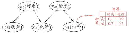
Example of a burglar alarm

The classic alarm network can be described in five variables: earthquakes. $E$Theft $B$The alarm. $A$John called. $J$ Call Mary. $M$。

graph TD
    E[Earthquake] --> A[Alarm]
    B[Burglary] --> A
    A --> J[JohnCalls]
    A --> M[MaryCalls]

The network is distributed as follows:

$$ P(E, B, A, J, M) = P(E)P(B)P(A \mid E, B)P(J \mid A)P(M \mid A). $$

If you specify five sets of local probability, you can paint the entire system. More importantly, the figure also tells us which variables can be ignored after the given evidence.

D-Definition and conditions independence

D-Segment(D-Separation) is the graphical rule for the independence of the conditions judged in DAG. It is structured around three basic structures:

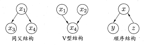
It's okay.

$$X \to Y \to Z$$

Not given $Y$ , the information can be passed along the path; given $Y$ Then the path was blocked, so... $X \perp Z \mid Y$。

Branch

$$X \leftarrow Y \to Z$$

$Y$ Yes. $X$ and $Z$ Common cause. Unobserved $Y$ , which are usually relevant; control $Y$ The blogger says:$X \perp Z \mid Y$。

Convergence

$$X \to Y \leftarrow Z$$

No observations. $Y$ The first is the "Standards of the Earth":$X$ and $Z$ Marginal independence; once observed $Y$, the path is activated, and the two reasons are relevant. This phenomenon is calledEmpirical(Explaining Away): For example, if an earthquake is found to have occurred, the need to alert the police is reduced by theft.

Learning and extrapolation

The Bayesian network has two levels of learning:

Parameter Learning: An estimate of the probability of conditions at each node when the chart is known to be structured. The discrete variable can be estimated to be the largest possible number:

$$ \theta_{ijk}^{MLE}=\frac{N_{ijk}}{\sum_k N_{ijk}}. $$

Dirichlet is used to smooth first when data is thin:

$$ \theta_{ijk}^{Bayes}=\frac{N_{ijk}+\alpha_{ijk}}{\sum_k(N_{ijk}+\alpha_{ijk})}. $$
Structural learning: Finds a suitable DAG from the data when the structure of the chart is unknown. This is a NH-Hard problem, and the common routes include:
- (a) A restraint-based approach: the use of independent testing of the conditions for the construction of the skeleton, such as the PC algorithm;
- (a) A rating-based method: use BIC, BDeu and other rating functions to support mountain climbing or Tabu Search searches;
- Mixing method: The pool of candidates is reduced by binding method, followed by statutory scoring, e.g. MMHC.

At the inference stage, the target is usually to calculate the probability of searching under evidentiary conditions, for example, $P(\mathbf{Q}=\mathbf{q}\mid\mathbf{E}=\mathbf{e})$I'm sorry. Accurate solvers can be found when the network is smaller; similar methods such as Gibbs sampling are commonly used when the network is dense or larger.

There's a dynamic map: The Invisible Markov model

The static Bayesian network has a set of variables discussed at the same time, and many data are naturally time-series.The Cain Markov model.Hidden Markov Model, HMM is the most classic and restricted form of the dynamic Bayesian network: it produces observation sequences using a hidden state chain.

Model definition

HMM contains two-layer random processes:

Invisible status sequence $Q={q_1,q_2,\dots,q_T}$: the true state of the system, which is not normally directly observed;
Observation sequences $O={o_1,o_2,\dots,o_T}$: Data available at every moment.

A discrete HMM usually says $\lambda=(N,M,A,B,\pi)$：

Status set $S={s_1,\dots,s_N}$；
Observation cluster $V={v_1,\dots,v_M}$；
State Transfer Matrix $A=[a_{ij}]$, of which

$$a_{ij}=P(q_{t+1}=s_j\mid q_t=s_i);$$
Launch probability matrix $B=[b_j(k)]$, of which

$$b_j(k)=P(o_t=v_k\mid q_t=s_j);$$
Distribution of Initial Status $\pi=[\pi_i]$, of which $\pi_i=P(q_1=s_i)$。

It relies on two key assumptions:

Zhith Markov's hypothesisThe current state of secrecy depends only on the state of secrecy of the previous moment.

$$ P(q_t\mid q_{t-1},o_{t-1},\dots,q_1,o_1)=P(q_t\mid q_{t-1}); $$
Observation independence assumptions: Current observations rely only on the current state of concealment,

$$ P(o_t\mid q_T,o_T,\dots,q_1,o_1)=P(o_t\mid q_t). $$

Three core issues

Probability calculation: Forward algorithm

Give model and observation sequences, calculation $P(O\mid\lambda)$I'm sorry. The complexity of all hidden sequences directly enumerated is $O(N^T\cdot T)$, the forward algorithm reduces it to $O(N^2\cdot T)$。

Define forward probability:

$$ \alpha_t(i)=P(o_1,\dots,o_t,q_t=s_i\mid\lambda). $$

Gradually:

$$ \alpha_1(i)=\pi_i b_i(o_1), $$

$$ \alpha_{t+1}(j)=\left[\sum_{i=1}^N\alpha_t(i)a_{ij}\right]b_j(o_{t+1}), $$

$$ P(O\mid\lambda)=\sum_{i=1}^N\alpha_T(i). $$

Decoding: Witterby algorithm

Give a view sequence to find the most likely hidden path:

$$ Q^*=\arg\max_Q P(Q\mid O,\lambda). $$

The Witby algorithm retains the best path to each state. You're the one who's gonna get you. $\delta_t(i)$ Means at the moment $t$ in $s_i$ , the maximum path probability is:

$$ \delta_1(i)=\pi_i b_i(o_1), $$

$$ \delta_t(j)=\max_{1\le i\le N}[\delta_{t-1}(i)a_{ij}]b_j(o_t). $$

And record the best forwards of every step. $\psi_t(j)$, the whole state sequence is restored by retroactive return after the maximum value of the endpoint is obtained.

Learning: Baum-Welch Algorithm

If only the observation sequence is not indicated in the hidden state, it needs to be estimated $A$、$B$ and $\pi$I'm sorry. Because the model contains hidden variables, it is not possible to complete a normal, very similar estimate directly; special cases of HMM using the EM algorithms -Baum-Welch algorithm。

E step calculation:

$\xi_t(i,j)$: Time $t$ As Status $i$ and $t+1$ As Status $j$ (b) the probability of a post-test;
$\gamma_t(i)=\sum_j\xi_t(i,j)$: Time $t$ Status $i$ - The probability of a posteriori.

M step by step to update transfer probability and launch probability in the expected number:

$$ \hat{a}{ij}=\frac{\sum{t=1}^{T-1}\xi_t(i,j)}{\sum_{t=1}^{T-1}\gamma_t(i)}, $$

$$ \hat{b}j(k)=\frac{\sum{t=1,o_t=v_k}^{T}\gamma_t(j)}{\sum_{t=1}^{T}\gamma_t(j)}. $$

Example: word type

In word type labels, word series are observations and word type labels are hidden. The probability of a shift between word-types and word-types is estimated at the time of training; the most likely word-type sequences are recovered from the sentence using the Witby algorithm at the time of projection. While many modern missions have used RNN, LSTM or Transformer, HMM is an important starting point for understanding serial probabilities modelling, dynamic planning and learning about hidden variables.

No direction: Markov follows the airport

When the relationship is symmetrical and does not have a clear causal direction, the no-go map is more natural.Markov follows the airport.(Markov Random Field, MRF) is particularly appropriate for expressing local correlations between image pixels, space units or network neighbours.

Figure separation and global marcroft

MRF uses no-go map $G=(V,E)$I'm sorry. Gathering Nodes $A$、$B$、$C$, if $C$ Blocked the drawing from $A$ Present. $B$ All the paths, then:

$$ A\perp B\mid C. $$

It's calledThe Global Marcov NatureI'm sorry. Unlike D-division of DAG, there is no need to address the observation of V-type structures in the unwinding map; the separation of the diagram itself gives conditional independence.

Group, Fist and Gibbs Distribution

No Flow byCorps(Clike) Expresss a partial interaction. If a strictly correct distribution meets the Marcov properties of the diagram, Hammersley-Clifford ensures that it can be written as a product of a large grouping function:

$$ P(X)=\frac{1}{Z}\prod_{C\in\mathcal{C}}\psi_C(x_C). $$

Of which:

$\mathcal{C}$ It's a huge gathering.
$\psi_C(x_C)\ge0$ is a dynamic function that measures the compatibility of the state of the variables within the group;
$Z$ It's a sub-function, which is the function of the sub-function:

$$ Z=\sum_x\prod_{C\in\mathcal{C}}\psi_C(x_C). $$

If you order $\psi_C(x_C)=\exp(-E_C(x_C))$, and get energy form Gibbs distribution:

$$ P(X)=\frac{1}{Z}\exp(-E(x)). $$

The lower energy state is more likely, which also connects probability-mapping models to statistical physics.

Ising Models and Images Go Noise

Ising Model is the simplest pair of MRFs. Make every node $x_i\in{-1,+1}$, whose energy function can be written as:

$$ E(x)=-\sum_{(i,j)\in E}J_{ij}x_ix_j-\sum_{i\in V}h_ix_i. $$

The first encourages the alignment of values at adjacent nodes, the second expresses that individual nodes are affected by external information. When using a binary image to go to noise, you can order $y_i$ For the noise pixels,$x_i$ For recovery pixels:

$$ E(x,y)=-\beta\sum_{(i,j)\in E}x_ix_j-\eta\sum_{i\in V}x_iy_i. $$

Minimize energy equivalence for the search for maximum back-probability (MAP) resolution: preserves the local smoothness of the image without detaching from the pixels observed.

Insumption and Gibbs Sample

The difficulty of MRF is the split function $Z$ Usually you need to list all the variables. If there is one, $N$ A binary variable, sum size is $2^N$, precise extrapolations quickly become unfeasible.

MCMC can avoid direct calculations. $Z$I'm sorry. In particular, in Gibbs samples, the full probability of a variable depends only on its neighbour:

$$ P(x_i\mid x_{-i})=P(x_i\mid x_{\text{neighbors}})=\frac{\exp(-E(x_i,x_{\text{neighbors}}))}{\sum_{x_i'\in Val(x_i)}\exp(-E(x_i',x_{\text{neighbors}}))}. $$

The attribute is offset by the molecule and the denominator. When the actual sample is taken, the individual node is updated repeatedly from the random starting value, with a conditional distribution; after the chain has constricted, the sample can approximate the target distribution.

Text Generation Diagram: LDA Theme Model

The first three models show static dependence, time dependence and local inactivity respectively. They also lay down the tools needed to understand more complex models: to break into joint distributions by graphics, to express invisible structures by hidden variables, and to re-establish them by approximate inferences.Potential Delicré distribution(Latent Dirichlet Allocation, LDA) bringing these ideas to the text would naturally constitute the last stop of this probability map model.

From wordbags to generating models

The simplest way to process text dataWordbag model(Bag-of-Words, BoW). It ignores the words and syntax, and records only the words that appear in the document and the frequency of each. BoW can convert text to vectors without being able to explain directly the semantic structure behind the document. Intuitively, an article is organized around several themes, each of which tends to use a specific set of terms.

Theme Model(Topic Mode) Writes this instinct into a generation process: the document selects the subject, the theme then the word. IDA is the classic model of it. It uses a flow map to indicate the generation relationship between variables, submersible variables to carry the theme structure in the document that cannot be directly observed, and a double plate compression to indicate the location of the entire document and the word.

Beyes Perspective: Dirichlet Co-examining

Before entering the LDA structure, the probability component used by it needs to be understood. When a single subject or word is sampled in a single location, a classification distribution (Categoric Distribution) is used; multi-scale distribution (Multilingual Distribution) is used to read the number of multiple samples together. The probability vector behind both can be used. Dirichlet DistributionAs a priori.

In PLSA (Probabiliistic Late Security Analysis), the subject proportion of the document is usually used as an estimation parameter. LDA uses Beyers Modelling: Documentation - Theme Distribution $\theta_d$ and theme-word distribution $\phi_k$ It's a random variable, and it's subject to Dirichlet's first test.

Classification/multiple distributionDescribe the selections made in a discrete group, and the number of counts obtained after multiple selections;
Dirichlet DistributionDescribe the probabilistic vectors corresponding to these discrete categories;
Dirichlet is classified/multiple distributionCo-protestThe posterioris therefore remain within the Dirichlet distribution group.

Co-benefits do not automatically make all late counting simple, but it allows us to decipher parts of the continuum, which makes it possible to fold Gibbs later.

Generate Process and Plate Notation

LDA describes the language library as a layered generation process from the subject scale to the specific vocabulary.

Core Variables

Document: Language library contains $D$ Part of the document, No. $d$ - Yes, I do. $N_d$ (a) Words;
ThemeOther Organiser $K$ Theme, word distribution for each theme $\phi_k$ Define in Size $V$ on the glossary;
Document Theme Scale：$\theta_d$ Representing documents $d$ Yeah. $K$ (a) The mix of the themes;
Theme Assign：$z_{d,n}$ Representing documents $d$ Medium $n$ (a) The theme of the choice of the word location;
Observation term：$w_{d,n}$ is the word actually observed at that location.

Figure structure

graph TD
    subgraph Plate_K [K Topics]
        beta((beta)) --> phi((phi))
    end

subgraph Plate_D [D Documents]
    alpha((alpha)) --&gt; theta((theta))
    subgraph Plate_N [N_d Words]
        theta --&gt; z((z))
        z --&gt; w((w))
        phi --&gt; w
    end
end

style w fill:#ddd,stroke:#333,stroke-width:2px

$w$ (a) is the actual word in the observation variable, the counterpart library;
$z$、$\theta$ and $\phi$ is the subvariant or unknown random amount to be extrapolated;
$\alpha$ and $\beta$ It's a pre-checked hyper-parameter to control Dirichlet;
Two layers of Plate indicate that the same generation steps are repeated for " for each document " and " for each word position in the document " , respectively.

Generate stories

For each theme $k \in {1, \dots, K}$From a priori $\operatorname{Dir}(\boldsymbol{\beta})$ in sample theme - word distribution $\phi_k$。
For each document $d \in {1, \dots, D}$From a priori $\operatorname{Dir}(\boldsymbol{\alpha})$ Medium Sample Document - Theme Distribution $\theta_d$。
Against Documents $d$ , and then click the $n$：
- From $\theta_d$ Medium Sample Theme Assign $z_{d,n}$；
- Distribution of words from the subject $\phi_{z_{d,n}}$ Medium sampled observation term $w_{d,n}$。

From the dependency of the conditions in the figure, the complete joint distribution can be broken down into:

$$ P(\mathbf{w}, \mathbf{z}, \boldsymbol{\theta}, \boldsymbol{\phi} \mid \boldsymbol{\alpha}, \boldsymbol{\beta}) = \prod_{k=1}^K P(\phi_k \mid \boldsymbol{\beta}) \prod_{d=1}^D \left[ P(\theta_d \mid \boldsymbol{\alpha}) \prod_{n=1}^{N_d} P(z_{d,n} \mid \theta_d) P(w_{d,n} \mid \phi_{z_{d,n}}) \right]. $$

It is not necessary to write each of these conditions in the natural language description: the process of generation is already given together with the breakdown of the figure and factor.

Insumption: folding Gibbs sample

When training LDA, only words are actually observed $\mathbf{w}$I'm sorry. Target is to assign the theme by the language library back. $\mathbf{z}$, the document theme ratio $\boldsymbol{\theta}$ and theme word distribution $\boldsymbol{\phi}$, which means a posteriori:

$$ P(\mathbf{z}, \boldsymbol{\theta}, \boldsymbol{\phi} \mid \mathbf{w}, \boldsymbol{\alpha}, \boldsymbol{\beta}). $$

This posteriori sub-consolidation constant requires the sum of a large number of hidden variables or points, which cannot be calculated directly. Similar to the previous MRF, LDA usually relies on approximation. Using Dirichlet co-relationship, you can use continuous variables $\boldsymbol{\theta}$ and $\boldsymbol{\phi}$ Parsing fractions, assigning only to discrete themes $\mathbf{z}$ Sample, therefore calledCollapse Gibbs Sample（Collapsed Gibbs Sampling）。

Sample formula

To simplify marking, assuming $\alpha$ and $\beta$ is the symmetric parameter for the pre-test of Dirichlet. Assign theme to all other word positions, current word $w_{d,n}$ Allocation to themes $k$ The probability of a condition is:

$$ P(z_{d,n}=k \mid \mathbf{z}{\neg(d,n)}, \mathbf{w}, \alpha, \beta) \propto \left(n{d,k}^{\neg(d,n)}+\alpha\right) \frac{n_{k,w_{d,n}}^{\neg(d,n)}+\beta} {n_k^{\neg(d,n)}+V\beta}. $$

Of which:

$n_{d,k}^{\neg(d,n)}$ is the document after excluding the current position $d$ to the theme $k$ the number of words;
$n_{k,w_{d,n}}^{\neg(d,n)}$ It's the word after the current position is excluded. $w_{d,n}$ Allocation to themes $k$ Number of times;
$n_k^{\neg(d,n)}$ is all allocated to the subject after excluding the current position $k$ the number of words;
The first bias is a topic already common in the document, the second tends to generate the subject of the current word.

The complete probability of the side of the document also contains the denominator $N_d-1+K\alpha$But it's all the subjects that are candidates $k$ It's all the same, so it's in this positive pattern.

Algorithms process and parameter restoration

A random initial theme is assigned to each word position in the language library.
Repeatedly through all word locations:
- Remove the theme assignment from the count of the current position;
- (a) Calculate its weight as a matter of subject matter based on the probability of the above conditions;
- Sample new themes with a centralized weight and update the count.
The preheating samples that have not yet been pre-dumped are discarded and the following samples are used to estimate the thematic structure.

When the sample is stabilized, the document - the theme distribution and the theme - the word distribution - can be restored by smooth count:

$$ \hat{\theta}{d,k}=\frac{n{d,k}+\alpha}{N_d+K\alpha}, \qquad \hat{\phi}{k,v}=\frac{n{k,v}+\beta}{n_k+V\beta}. $$

Thus, the result of LDA is not just a theme label for each document, but rather a mix of documents on multiple themes and a probability distribution of the vocabulary for each theme.

Summary: from chart structure to generation model

The unified idea of the probability map model is:Quantification of uncertainty by probability, using graphics。

Bayesian Network(a) The use of DAG as a static condition depends on the direction of decomposition with joint distribution and changes independent relationships through D-division of research evidence;
HMM(a) The structure of the direction is extended over time, describing the generation and evolution of the sequence in a hidden state;
MRF(a) a local interaction of symmetrical symmetry with no directional charts, groups and force functions;
LDAA replicated orientation generation structure with Plate combines submersible variables, co-prospect and approximate extrapolations into text theme modelling.

The four models are not an upgraded version of each other, but are extended on different data structures in the same model language: static variables, time series, spatial domains and text collections, where conditions can be determined independently, and the joint distribution can be broken down and extrapolated algorithms selected.

And the route to LDA is also a complete closed ring. After reading the correspondence between maps, joint distribution and post-pregnation, and in the face of a new probability model, it is not necessary to remember only the algorithm name, but to ask three more stable questions: What variables can be observed, what structures are hidden, and what dependencies are generated by data. LDA is fit to end it because it is not just another subject algorithm, but rather centralizes the core components of the Probability Map model into the same example.

Extending reading

Machine Learning Introduction and Monitoring Learning: The Bayesian Catalogue: understand why the chart model expresses the dependency of attributes from plain/semi-supra.
Karman filter family: KF, EKF, UKF and EnKF: Recursive estimation and filtering routes in continuous status space.