Exploratory Data Analysis: Descriptive Statistics, Visualization, and Preprocessing

This English version was machine-translated from the Chinese original. Technical terms may require verification.

Overview of exploratory data analysis ideas

What's the data analysis?

Data analysis It's a new direction in statistics.

• It does not require us to give an accurate measure of the uncertainty of the method, which is indispensable in the estimation of parameters in classical statistics and in the hypothetical tests;
• It values the anti-disturbability of the method and its effectiveness at the same level.

Existing mathematical statistics attach great importance to measurement uncertainty, but they tend to rely on assumptions for this precise measure, which then leads to the theory of mathematical statistics being applied lightly;

The emergence of data analysis is a change in the idea that we have shifted the focus of our work to making the data talk, processing our data in some less formal ways, providing a basis for the subsequent stage of validation, without considering the precise measure of their uncertainty.

— Chen Chi-Yu — Explored data analysis in Chinese

What is exploratory data analysis?

Simply put, exploratory data analysis is a bridge between classical statistical analysis and popular data mining and machine learning (also those parts of classical statistical modelling).

He's the only thing that makes us understand the data, the data from different angles.

EDA (exploratory data analysis) is an emerging part of statistics with the relative concept of CDA validation data analysis

Data analysis is in two stages, exploratory and authentic, and we can only give the right results in alternate use.

This exploration does not prejudge ideas and assumptions, but rather wishes to use the results of exploration to present some ideas and assumptions for subsequent modelling, i.e. CDAs, which are inseparable.

It's obvious that the EDA should be a non-parametric approach.

What's in the EDA?

Scientific visualization is an important part of the EDA. R Statistical visualization in which separate presentations are made

Descriptive statistics are the subject of an introduction to statistics, and we do separate studies, descriptive statistics and visualization, and we could have classified them all in the EDA.

The major part of probability density estimates is presented in descriptive statistics. As far as further validation is concerned, it falls within the category of non-parametric statistics, which can be read in conjunction with the distributional shape in visualization.

Pre-processing of data should also be part of the EDA, which is the basis for subsequent data analysis and will be presented separately later in this paper.

In addition, feature engineering is an important pre-treatment method in the field of machine learning, which includes features screening, feature construction and downscaling.

Characteristics of exploratory data analysis

According to David and Tukey, underwriting Robust and Exploratory Data Analysis, an exploratory data analysis was presented.

In the current industry, Robust has been translated into greatness, and Professor Chen has been translated into resistance, and sometimes we also call it robustness, and here we do not dwell on the details of translation, which is central to it.

Validity requires that data analysis methods are insensitive to the local poorness of the data, which is local, but can change dramatically.

So what's the connection between exploratory data analysis and robustness? Validity and exploratory data analysis are holistic rather than explicit. All exploratory data analysis methods should be as insensitive as possible.

Therefore, the use of fractionals as a representative of high robust digital characteristics in the EDA is very extensive, including five-digit synopsis, box lines, differentials, and so on.

Know our Data

Descriptive statistics

Descriptive statistical analysis is the most basic way of understanding data.

Data visualization

Besides, data visualization is an important part of the EDA. R Statistical visualization

Data preprocessing

Basic introduction to data pre-processing and frequently asked questions

Basic description of pre-processing data

Before we start, let's get a picture of the entire data mining process.

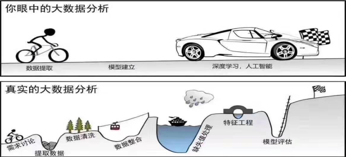
Pre-processed data are the most basic elements of data mining, but it also happens to be the most time-consuming part of data mining, the more vulnerable part of data science platforms such as Kagle, which contains a lot of work.

Data and features determine the upper limit of machine learning, and the selected models and algorithms are just going to approach the upper limit.

Common issues in data preprocessing

Here's why we're doing pre-processing.

For data objects, we can obtain unprocessed features (attributions), which may be the following:

• Not part of the same schematic: the specification of the characteristic is different and cannot be compared together (uniform unit)
• Information redundancies: For certain quantitative features, the useful information contained is compartmentalized, such as learning achievement, and if only “failure” or “failure”, then quantitative scores need to be converted to “1” and “0” for pass and failure (quantitative characterization)
• Qualitative characteristics cannot be directly used: some machine learning algorithms and models can only accept input of quantitative features, and then the qualitative features need to be converted to quantitative features (Qualitative Quantification)
• Missing value: missing value needs to be supplemented (missing)
• When data dimensions are too high, there is also the problem of what is called "Curse of Demensionality" (data down) We'll stay on the feature project and discuss the data downs and downs in the feature project.

Feature extraction and type conversion

Data are first required for pre-processing. The large amount of data obtained in experimental or operational systems is often not directly relevant to research issues and is often unstructured. At this point, the first step in the data mining exercise is to be carried out: feature extraction and type conversion.

Create a set of feature data that can be used by analysts to convert feature data to a uniform expression

The way in which the feature extraction takes place depends on the problem we're dealing with, and often also on the experience of analysts.

Source Data Type	Target data type	Methodology
Numeric Type	Type	Separated
Type	Numeric Type	Binary
Text	Numeric Type	Potential semantic analysis (LSA)
Organisation	Disconnected sequences	Symbol Convergence Approximation (SAX)
Organisation	Multi-dimensional Numeric	Dispersed small wave transformation (DWT); discrete Fourier transformation (DFT)
Disconnected sequences	Multi-dimensional Numeric	Dispersed small wave transformation (DWT); discrete Fourier transformation (DFT)
Space	Multi-dimensional Numeric	DWT
Figure	Multi-dimensional Numeric	Multi-dimensional scale (MDS); image conversion
Any type	Figure	Similar figure (limited availability)

As a matter of strong empirical reliance, there is no introduction to the fact that we have our own programs in different fields, no common methodology.

Complex feature breakdown

Some feature fields may include a large amount of information, such as a field containing the time and time of the year in which our valuable information is hidden, but cannot be used directly, which is the problem of decomposition of complex features.

String Split: In the case of the Titanic data sets, the class number C123 indicates the passenger identification information from which the information from the C-class is likely to be effective for predictions, which is the string split.

Timetamp SplitDepending on how we feel, consider which of the time-spans of the year to keep, such as four seasons, working days and rest days, etc.; if there are time-zone information, there is also a need to consider how to harmonize them, while time-zone information can also reveal geographic information as an independent feature.

Location Information SplitLongitudes, countries, etc. are part of the location-segregation information; we often wish to consider longitudes separately, so that they generally have a better effect.

Common data pre-processing methods

We'll be back with the data pre-processing approach below, which must not be complete, because many of the methods are taught in other courses.

• Data cleansing: missing certain log values for data cleansing processing data, noise in smoothing data, detection of anomalies, correction of inconsistencies, etc.
• Integration of data: Integration of data from different sources of varying quality. Good data integration reduces redundancy and inconsistency in data, thereby increasing the accuracy and speed of subsequent steps
• Data conversion: conversion of data into forms applicable to data mining through smooth aggregation, data overview, standardization, etc.
• Data downside: to translate high-dimensional data into low-dimensional data and to maintain most of the information in the original data, so that data mining results are the same or almost the same as pre-downgrade results

Relevant theoretical support

Code Relationship Algebra 3The data is sorted out to make sense of the structure of the data.Which means...

• Each feature is in one column.
• Every example is in one line.
• Each feature should have only one table.
• If the features are in multiple tables, then there's a column that connects them. That's why we're compiling the data.

Data Cleaning

Let's just talk about what needs to be done.

Missing value processing

Missing values are an unavoidable problem in actual data, and different strategies should be adopted for different data scenarios, starting with the distribution of missing values.

• If the missing value is minimal and this dimension is not important, normalDeleteThey have little impact on the overall data situation;
• If the missing value is higher or the information on this dimension is still important, the immediate deletion will have a bad effect on the results of the algorithm run behind, and we need to consider plugging data.

Losses generally fall into three categories.

• Total random missing MCAR (and any other variables unrelated to yourself)
• Random missing MAR (misses associated with other observation variables)
• Non-random missing MANR (misses associated with their own extraction)

Of these, MAR is the most common, and we generally assume that this is the only way to do it on the basis of modelling plugs.

Average or Middle Fill

It will not reduce sample information and process simple, but will cause deviations when missing data are not random; For normal distribution data, the average can be used instead, and if the data are tilted, the median may be better used

Integrating technical thinking

• Random plug-in - random extraction of a sample from the general population in lieu of missing samples;
• Multiple plug-in methods• Forecasting missing data through the relationship between variables, such as the use of the Monte Carlo methodology to generate complete data sets and, finally, to aggregate the results of the analysis,It's a relatively robust plug-in technique, highly recommended.
• Thermal platform plug-in -- find a sample similar to the missing value in the non-missive data cluster (symmetry sample) and use the observations in it to plug in the missing value, that is, $k$Next plug.

Modelling plug-in technology

It could be determined by means of a process based on reasoning such as return.

For example, using the properties of data centralizing other data, a determination tree (return equation) can be constructed to predict the value of the missing value

Multi-plugging (Multiple Imputation)

Retain Missing Technology

• In the case of classification problems, the missing can be used as a category
• If the model is willing to accept the existence of NA, retain NA as the missing embedded model to the back

Missing is sometimes information.

For random absences, we can only deal with by plug-in. However, there are many problems involving the extraction of data that are not pure, the absence of regularity in many cases, such as those resulting from a failure in the work of an operational component, the lack of the means of data collection itself, and, if the reasons for the absence can be identified, we can re-target the processing of data to fill the gaps, and sometimes even the lack of data can be extrapolated very reliably through other available data.

Sometimes the lack itself is an information to consider. It would also be valuable to include the missing themselves as information in the model, and the absence of some data implied the characteristics of the users themselves.

Treatment of anomalies

Unusual values are also commonly referred to as “outlier”, i.e. points that are not consistent with the general behaviour or characteristics of other sample points in the sample space. In general there may be the following causes:

• Error in calculation or error in operation (miscal data)
• The variability or elasticity of the data itself (real special data)

Disconnection points may not necessarily be useless data, but they may be of interest to users, for example in the area of fraud detection, where those that are inconsistent with normal data behaviour tend to signal fraud and thus become a concern for law enforcement.

We're not the only ones dealing with detached values.

• De-grouping is the most common method of processing
• If we really want to keep this sample, we usually use a plug-in that's considered missing.
• If algorithms aren't sensitive to entanglement, it's okay not to process entanglement values.

Statistically based discrete site testing

Such tests assume that all data in the sample space are consistent with a distribution or data model, or Discordancy test (discordancy test) Points

Normal distribution$3\sigma$ Principle. Use of box-line maps for detached site detection.

Distance-based isolation site testing

Just as we conduct cluster analysis based on distance, those isolated categories can be considered as discrete points. Here, reference can be made to machine learning about distance calculation and hierarchy. In practice, those points that are too far away from the other points are considered separate points.

Density-based isolation site testing

Similarly, discrete points can be understood from the point of view of density clusters. In practice, those too low-density points are considered discrete. This method detects both global and local detached sites.

Data heavy.

Repetition of data is common in practice, and in some data mining models these redundant data increase the difficulty of data analysis and processing speed, and therefore data need to be addressed Heavy

There are common ways.

• Cross-referenced data search — highly complex, only in smaller data situations
• Hash stated that - generating data fingerprints, simple and efficient, applicable to large-scale data, represents algorithms:
  • Bitmap: Bitmap method;
  • SimHash: similar to Hashi;
  • Blom Filter

Many models don't need data to work hard.

Data to Noise

Noise, a random error or equation of the measured variable; most data mining methods treat discrete points as noise or anomaly, but there are data mining methods that specifically study noise

Observation = True Data + Noise

The usual data-noise methods are:

• Boxing method: Checking data “neighbor” (i.e., surrounding values) for smooth and orderly data values
• regression method: smooth data using a function that combines data to help eliminate noise

Most models (especially statistical models) don't need data for noise work.

Manually remove useless features

The manual removal of useless features is highly dependent on our experience, and here is a summary of some basic experiences. It was removed from the perspective of the data itself, and those business-based manual filter features could not be described here:

• Delete a clear non-functional amount: if the number of the observation is used, there is no theoretical positive effect on the model
• Delete the amount of excess of the missing value ratio: no fixed line, depending on the circumstances
• Removes the feature of a difference of almost zero:
  • The number of variable values is less than 10% of the variable.
  • Biggest two withdrawals of frequency, frequency ratio above 20%.
• Delete the compound linear amount:
  • Found the two strongest variables of the current correlation coefficient
  • Calculate the relevant coefficients for them and for the rest of the population (combinant coefficients)
  • Delete the largest variable of the compound coefficient
  • Whether this step needs to be repeated and continued to be deleted, depending on the data set
• Screening based on relevant coefficients to retain more relevant quantities (seeDescriptive statistics and visualization: related analysis）

Data Integration

We're still introducing what we need to do.

Data integration integrates data of different kinds from different sources. Good data integration reduces redundancy and inconsistencies in data

In practical use, data integration is often determined by data, for example: Entity Identification Project: trying to match the records of different data sources pointing to the same entity in the real world.

There's more to it.

Data Conversion

The purpose of the data conversion is to move data from one form of expression to another and to meet the conditions for data mining.

And here we're presenting some of the more basic data conversion methods, which in fact has become a subject in statistics, with a lot of research.

Common data conversion methods can be broadly grouped into the following categories:

• Separated
• Binary
• Harmonization and standardization
• Feature Encoding

Separated

Some data mining algorithms, in particular some classification algorithms, require that data be in the form of classification attributes or that classification forms be effective in increasing the efficiency of algorithms

In this way, continuous properties often need to be converted to classification properties (dissemination, disscretion) and continuing and discrete properties may need to be converted to one or more binary properties

Common discrete methods include:

• No monitoring: boxing method (separate/equivalent), visual division, median grouping, etc.
• Supervision: Chimerge Law MDPL Law, CAIM Law, etc. Monitoring separation is a good method for FE workers who lack intuitive and field knowledge

We've told you to be careful.R Discussion on statistical visualization of careful data processingBut at this point, we have to be separated. Just be vigilant.

A customary rule of the boxing method is:

• The number of groups between 5 and 20, the number of data in groups.
• Group spacing as far as possible (except when equal frequency groups)
• The group distance selects the odd number as far as possible, but even if it's the case.
• The maximum group ceiling covers all individuals, but avoid too many spills as much as possible.
• Avoid the use of groups with upper or lower limits

Binary

Characteristic dualisation is the process of converting a numerical feature to a boolean value, the core of which is to set one Threshold, with 1 value greater than the threshold and 0 value less than the threshold

Harmonization and standardization

Normalization is a simple calculation, with a schematic expression transformed into An expression with no scalding, becomes the cursor

Standardization aimed atHarmonization of data profiles Increase the interpretability of algorithms, and at the same time, in those algorithms that require a gradient decline, the uniform scale helps to accelerate the reduction of gradients.

In traditional machine learning and statistics, integration and standardization are essential; in the field of in-depth learning, we have also developed more methods of neutralization to help implement the declining gradients.

There are common ways.

• Based on polarization:$\hat{x}=\frac{x-x_{\min}}{x_{\max}-x_{\min}}$ It causes the anomaly to be squeezed into a small compartment, so it should be done after processing the anomaly.
• Maximum unified absolute value:$\hat{x}=\frac x{x_{\max}}$
• z-scores convert:$\hat{x} = \frac{{x-\mu}}{\sigma}$
• Ten times zoom: $hat==<1$
• Robust scaling ：$x_{scaled}=\frac{x-median(x)}{IQR}$
• Paradigm homogenization:$\tilde{x}=\frac{x}{\left|x\right|_{2}}$

Data Merge

Dispersion reduces the size of the category by converting the data from continuous to multiple disaggregated indicators, and thus reduces the cost of modelling operations.

Data amalgamation is another fragmentation of discrete data. Sometimes there are too many categories of disaggregated data and there may be hundreds of them, so that the use of characterization codes leads to too many variables.

The goal of data consolidation is to reduce the number of variable categories. Common methods include:

• Manual consolidation of certain categories based on our understanding of variables
• For those categories whose share is less than 20 per cent (customary rules), they are all merged into a OTHERS category, which can also be used as a supplement, i.e.Slight Category Merge

Feature Encoding

The feature coding is about the idea that the classification emerges from variables.

Characteristic tectonics: Crossing and coordinates

Characteristic tectonics refers to the processing of the original data based on experience and the acquisition of features that are more meaningful to the model. It requires you to spend a lot of time on sample data, thinking about the nature of the problem, the structure of the data and how best to use them in predictive models. Calculateable features mean the calculation after input of an existing feature and the result as a new feature. It is more applicable to simple ML models (e.g. linear regression interactives); neural networks are generally considered to be self-explanatory in the learning of calculable features, although the introduction of calculable features into NN can also enhance effects. In general, three types of questions are studied: single characterization transformation (see section on data conversion), characteristic algorithm combinations, and the conceptual transformation of feature coordinates.

Characteristic algorithm combination: The algorithm combination of features is also called"Multiple Characteristics"I don't know. If a combination of characteristics is meaningful in the problem area, it can be significantly added. For example, if there are two characteristics: length and width, the size (long times width) has the same effect. Adding such a combination would require a certain intuition, and adding all algorithmic combinations would be a mistake — because the characteristic combination is very large and should be guided by as much knowledge as possible.

Descartes.: If both characteristics are always present (e.g. floor and room numbers), the use of the two characteristics as a separate feature enhances the signal for the ML algorithm. It's the reverse of decomposing complex features.

Changing the concept of the feature coordinate system: If we think that two vector angles are meaningful, then the use of polar-coordinate systems can be considered to facilitate model learning of angle characteristics; if we want to reduce relevance, then the rotational-coordinate system completed from the Marseille distance can be considered. For color features, we also have RGB, HSV, etc., which have their own coding features.

Identity selection and learning

Feature selection selects a small number of useful features from a large number of featuresI don't know. Not all characteristics are equal: attributes that are not relevant to the issue need to be deleted, some are more important than others and others are redundant. Characteristic selection is the automatic selection of a subset of the most important features of the problem.

The role of feature selection is:

• Simplify models and increase their interpretability
• Reduction of training time
• Avoiding dimensions of disaster
• Improve model interoperability and reduce alignment

There are three main types of features selected:

• Embedd: the learning algorithm itself contains features selection steps, such as decision tree;
• (a) Encapsulation (wrapper): feature selection is integrated with the training process, and LVW (Las Vegas Wrapper) is used to perform characterizations with the result of a trained model;
• Filtering (filter): characterization selection is completely independent of training, selection is based on the characteristics themselves and is not related to a learning device.

Filter

The filter feature selection considers the link between the variable and the target variable to filter the feature, and the evaluation criteria are derived from the intrinsic nature of the data set itself. According to researchers, the more relevant features or feature sub-assemblies obtain a higher accuracy rate on the classification. The evaluation criteria selected for filter features are divided into four categories: distance measure, information measure, correlation measure and consistency measure.

Advantages: Algorithms are very common; training steps for taxonomics are omitted, and algorithms are of low complexity and therefore applicable to large-scale data sets; a large number of unrelated features can be quickly removed and pre-screeners as features are appropriate.

Disadvantages: Because the evaluation criteria are independent of specific learning algorithms, the selected feature subsets are generally lower than the Wrapper method in terms of classification accuracy.

Relief Method: Using the Relief method allows for steady filtering (filter); it is essentially studying relevance. The method was designed."Relevant statistics"to measure the importance of the characteristic. The statistical volume is a vector, each of which corresponds to an initial characteristic, while the importance of the characteristic subset is determined by the sum of the relevant statistical weights corresponding to each characteristic. Only one threshold will eventually be specified $\tau$, choose the match $\tau$ Characteristics corresponding to large relevant statistical weights are sufficient; the number of characteristics to be selected can also be specified $k$, select the statistical weight of the relevant statistics $k$ A signature.

This statistically relevant amount is calculated as: a given training set.1,y_1),(\boldsymbol{x}2,y_2),\ldots,(\boldsymbol{x}m,y_m)}$，对每个示例 $\boldsymbol x_i$，Relief 先在 $\boldsymbol x_i$ 的同类样本中寻找其最近邻 $xIt's called"Guessing the nearest neighborhood."(near-hit), from $x_i$ \bardsymbol{It's called"Wrong neighborhood."(near-miss) The relevant statistics correspond to properties $j$ . The value is $ \delta=sum}mathrm{diff} (x j), x i,\mathrm{j}^mathrm{diff} (x i^j}, x mathrm{nm}^j)^: of which $x_a^j$ For sample $x_a$ In Properties $j$ above the value,$\mathrm{diff}(x_a^j,x_b^j)$ Depends on properties $j$ Type: if discrete, $x_a^j=x_b^j$ 0, otherwise 1; if continuous, $|x_a^j-x_b^j|$I don't know. Attention. $x_a^j, x_b^j$ Regulated to [0,1] slots.

It's essentially a calculation of a characteristic in"Wrong guess."and"Yeah."Whether there is a clear difference between the two: if there is, there is an increase in the relevant statistical weight, and the final average of each sample is the final output. Relief, which is designed for the issue of the second classification, expands the variant Relief-F to deal with the issue of multi-classifications, although they have little effect on qualitative self-variant.

Seal

Wrapper features select the performance of learning algorithms to evaluate the merits of the feature subset. For the feature subset to be evaluated, the Wrapper methodology requires the training of a taxonomyr (which needs to be designated by a person) to evaluate the feature subset based on its performance.

Advantages: The feature subsets found by the Wrapper method are usually better classified than the Filter method.

Disadvantages: The selection of features for the Wrapper method is less common and requires a re-selection when learning algorithms are changed; because each evaluation subset is trained and tested with a taxonomy, algorithm calculations are highly complex, especially for large data sets, and are implemented for a long time.

Specific methods of encapsulation are often studied by means of search, such as:

• Recursive feature elimination method
• Back-and-back search methods for greedy thoughts
• Random Search Method

Stable Selection: Stability choice is based onSecondary sampling and selection algorithm (training model)In combination, the choice can be regression, classification SVM or similar algorithms. The principle is achieved: the training model is run on different feature subsets, repeats and eventually aggregates the results of the feature selection. For example, it is possible to measure the frequency of a feature considered to be an important feature (the number of times it is selected as an important feature divided by the number of times it is tested in its subset). Ideally, important features will score close to 100 per cent; slightly weaker features will score non-0; the least useful features will score close to zero. It's not especially steep, it's different from the results of pure LASSO and random forests, and it shows that stability choices are not the same.Overcoming aggregation and understanding of dataIt helps. In general,A good feature is not divided into zeros because of similar characteristics.I don't know. Stability choices are often one of the best performance methods in many data sets and environments.

Recursive Characteristic Elimination (Recursive Feature Integration, RFE)The RFE's main idea is to conduct multiple rounds of training using a base model (e.g., SVM or regression model): after each round of training, grade the lowest score on the basis of the coefficient of each feature, remove the smallest score, construct a new feature set with the remaining features, and conduct the next training round until all the features are over. The concrete steps are:

1. Repeated construction of models (e.g. SVM or regression models);
2. Selecting the best (or worst) features (based on coefficients) and putting aside the selected features;
3. Repeats the steps 1 and 2 above on the remaining features until all the features are over.

The order in which the features are removed in this process is the sort of characteristics that are actually a search.Best Feature SubsetThe greedy algorithm. The stability of RFE depends to a large extent on which model is chosen in the iterative selection:

• If ordinary returns are used, unregulated returns are unstable, and therefore RFE is unstable;
• If the Ridge or Lasso model is used, a regularized return is stable, so RFE is stable.

Characteristic Value SortingTheoretically, if, after sorting or disrupting a particular feature, the effect of the model (for both positive and negative) (forecast rating) is obvious, this characteristic can be shown to be important to the model; conversely, the absence of such a feature does not affect the model ' s effectiveness. Characteristic value sequencing is the method of design based on this idea.

Embedded

The embedded feature selection integrates the feature selection process with the learning device training process.They're done in the same optimisation.This means that characterizations are automatically made in the course of learning devices training. In the case of embedded methods, the best example of retrogression is:$L_1$ Rectification is easier to dilute, so it's usually based on $L_1$ Regularized learning methods are referred to as embedded feature selection methods, which are integrated and completed simultaneously with the learning device training process. Ridge, LASO, ElasticNet.Linear regression base。

In addition to being based on the idea of regularization, embedded characterizations based on tree models are commonly used: decision tree, gradient up tree are embedded characterizations.Deep learning is also an embedded feature selection method.。

Rare expression and dictionary learning

The issue of identity selection is characterisation."Rareness", i.e. many columns in the matrix are not relevant to the current learning task, removing these columns through feature selection, enhancing model effectiveness, interpretability and reducing the difficulty of training.

Now let's think of another sort of thinness:$D$ There are many zero elements in the corresponding matrix, but they do not exist as columns or rows. When samples have this thin expression, there are a number of benefits to the learning mission: highly thinness makes most problems linear, so SVM can have a good effect in this data; and, at the same time, thin samples do not create a huge storage burden, because the thin matrix already has a lot of efficient storage methods, so this is what we seek.

It's good for us to build a model.(Of course too thin data is bad). So, if you give a data set, $D$ Is it dense, i.e. ordinary, non-sorted data that can be converted into"Rare expression"(sparse representation) in the form of a rare advantage?

Obviously, there's no modern Chinese-language common vocabulary available for general learning assignments (e.g. image classification). We need to learn one of these."dictionary"A suitable dictionary was found for a sample of common dense expression, which was converted into a suitable form of thin representation, thus simplifying learning tasks and reducing the complexity of models. It's usually called"Dictionary Learning"(dictionary learning)"Rare Encoding"（sparse coding）。

given data set ${x_1,x_2,\ldots,x_m}$The simplest form of dictionary learning is $US$US$US$US$US$US$US$US$US$US$US$US$US$US$US$US$US$US$US$US$US$US$US$US$US$US$US$US$US$US$US$US$US$US$US$US$US$US$US$US$US$US$US$US$US$US$US$US$US$US$US$US$US$US$US$US$US$US$ $US$US$US$US$US$US$$US$US$US$US$US$US$US$US$US$US$US$US$US$US$US$US$US$US$US$US$ 2^2+\lambda\sumI'm sorry. of which $\mathbf{B}\in\mathbb{R}^d\times k$ As a dictionary matrix,$k$ The amount of vocabulary called dictionary is usually specified by the user.$\boldsymbol{\alpha}_i\in\mathbb{R}^k$ It's a sample. $x_i\in\mathbb{R}^d$ The thin expression. Obviously, the first thing to optimise is to hope that $\boldsymbol\alpha_i$ It's a good remodel. $x_i$The second is hope. $\alpha_i$ Try to be thin.

Data Transformation

In a lot of cases, we need to change the original data to better characterize the data; it's often because the original data has...

• Strong asymmetrical
• Mass Offset Values
• The idea of a simple model presents a large and non-accidental flaw.
• The median and four-point differentials derived from the box chart reflect their relationship. We want to make further analysis more rational by making some shape adjustments to the raw data. It's a very broad concept, and it's a constant, and it's an order, and it's a variation, but we're just going to look at one of the special variations that he's asking for.
• The median order remains unchanged
• Continuous and smooth functions
• The primary function can be constructed in the form of simple calculations. Change is a cost, not always a benefit.

& Change

The definition, the transformation, has the following expression. $T p(x)=\begin{cases}ax^p+b&,p\neq0\c\log x+d,p=0\end{cases}$$ 里面的参数可以比较自由的选取 但是需要保证满足我们前面要求的变换的性质 幂变换有下面三种比较常用的形式 $$T_p(x)=\begin{cases}x^p,&p>0\\log x~,&p=0\-x^p,&p<0\end{cases}.$$ $$T_p^*(x)=\begin{cases}\dfrac{x^p-1}{p},p\neq0\[2ex]\ln x&,p=0\end{cases}$$

Reason for the change.

Inline data requirements

For example, we sometimes want to turn degrees centigrade into fahrenheit, and to logarithmize population numbers, which are based on the characteristics of the data themselves, often relying on our experience with this type of data, and they can be useful for further analysis.

As symmetrical transformation

The graphs and the coefficients tell us whether there's a systematic bias in the data, which we don't usually want, so we need to study how the data is symmetrical.

• Basic, we'll try square root changes, which is... $p=\frac{1}{2}$
• If, however, there's not enough symmetry, we'll consider a logarithmic variant, which is... $p=0$
• The logarithmic variants can also be used. $p=\frac{1}{4}$Replace

To eliminate dependence on the quartile and median

Eradicating this dependency is often considered to be more appropriate for intuitive and exploratory analysis

To construct the approximate linear relationship of the variable

The approximation of linear models makes it easier to make simple drawings and analyze the differences.

When is it worth changing?

We don't have a strict standard.

• The maximum data value and the minimum data value are relatively large.
• There's a habit of changing things like this.
• It's much worse and it's a pattern.

Change the broadest application from custom.

Box-Cox Transformation

The point of Box-Cox transformation is to match the linear regression model in the front with all the assumptions we need. It includes the Gauss-Markov hypothesis. It's actually a way to fix the problem with regression diagnosis. Note that the Box-Cox transformation is not a single variant, but a variant. Overall expression of the Box-Cox variant $ \begin{array}&Y^{(\lambda)}=\begin{cases}\dfrac{Y^{\lambda}-1}{\lambda},&\lambda\neq0,\\ln Y,&\lambda=0, \end{cases} Obviously, the core of the Box-Cox shift is the right choice.$\lambda$ In fact, we don't have a way of getting a stable.$\lambda$ In practice, we choose a lot.$\lambda$ There's been a lot of Box-Cox conversions, based on a variety of information standards.

• Square difference
• Meet normality assumptions

Maze distance changes: Maze distance is achieved by European range following the rotation axis, which eliminates self-relevance

White

The Ma's distance shift eliminates self-relevance, the standardized shift changes the unit differences, and the combination of the two is bleaching.I don't know. The data generated by bleaching are well suited for modelling analysis of models, and more common methods of bleaching are PCA (main component analysis) and ZCA bleaching. Albinization is a way of changing data, but because of its advanced level, it is often discussed in feature projects.

In addition to bleaching, another common single feature conversion is the Sigmoid operation. It has an S-type function that preserves the variability of the intermediate part of the numeric domain and reduces the variability of both ends of the range: $$\frac{1}{1+e^{-x}}$$