Linear Regression Basics: Linear Models, Least Squares, and Diagnostics

This English version was machine-translated from the Chinese original. Technical terms may require verification.

Introduction

Linear statistical models are one of the most widely used models of modern statistics and are the basis for a very large number of statistical studies; because there are many linear dependencies in the real world and many dependencies that can be converted; linear models are very easy to build and process, and we present only a few simple examples in the introductory section to facilitate understanding of the various approaches behind us.

At the beginning of the introduction, we need to know the process and purpose of creating linear statistical models.

A linear statistical model would allow us to understand the relationship between the variables and the variables; to understand the potential linkages between the variables, and finally to use the models to achieve the prediction functions that we need most, decision-making, understanding linkages, etc.;

Of course, it's not that easy to build a model, and we need constant testing to correct the methods used before and until we're satisfied.

Return analysis is a classic statistical issue, and we should not lack statistical thought.Anscom Quartet

Linear regression model

A brief introduction.

In the real world, there are a lot of situations where two variables, like X and Y, have some dependencies, which X can partially determine the value of Y, such as height and weight, temperature and city consumption; we can't determine precisely (and the exact function is not the same).Relationship For the study of relationships, regression models are an important part.

In the example above, Y's response variable X's predictive variable, we know that part X determines Y, so we can give a model that includes both X-Y's decision and those factors that are not taken into account and random. $$Y=f(X)+e$$ Here.$f(X)$It's what makes decisions. $e$It's a random error.$E(e)=0$

When?$f(X)$Take Special Linear Functions$f(X)=\beta_{0}+\beta_{1}X$ At the time, we got a linear regression model that we're looking at here.$f(X)=\beta_{0}+\beta_{1}X+e$ It's a linear regression model.

After applying appropriate statistical methods to determine these regression factors, we call the result linear regression equations.

In practical applications, there's often more than one variable, so it's easy to give multiple forms of linear regression. $$Y=\beta_0+\beta_1X_1+\cdots+\beta_{p-1}X_{p-1}+e$$

Matrix

We...$n$The linear regression model of the dollar is performed.$n$Sub-observation. $$x_{i1},\cdotp\cdotp\cdotp,x_{i,p-1},y_i,\quad i=1,\cdotp\cdotp\cdotp,n$$ They're satisfied. $$y_{i}=\beta_{0}+x_{i1}\beta_{1}+\cdots+x_{i,p-1}\beta_{p-1}+e_{i} $$ Include Matrix {\cHFFFFFF}{\cH00FFFF} {\cHFFFFFF}{\cH00FFFF} {\cH00FFFF} {\cHFFFFFF}{\cH00FFFF}&x_{11}\cdots x_{1,p-1}\1&x_{21}\cdots x_{2,p-1}\\vdots&\vdots&\vdots\1&x_{n1}\cdots x_{n,p-1}\end{array}\right|,\mathbf{\beta}=\left|\begin{array}{c}\beta_0\\beta\mathbf{\lambda}\\vdots\\beta_{p-1}\end{array}\right|,\mathbf{e}=\left|\begin{array}{c}e_1\e_2\\vdots\\vdots\e_n\end{array}\right|,$$ 得 $$y=X\beta+e$ In the form of a matrix,$y$It's called the observation vector. $X$It's called Model Matrix. $\beta$Unknown parameter vector $e$A random error vector.

Random error generally requires the following conditions (Gauss-Markov hypothesis)

• $E(e_{i})=0$ Average error value is 0
• $Var(e_{i})=\sigma^{2}$ Error Equation
• $Cov(e_{i},e_{j})=0$Irrelevance of errors

A linear regression model

For Functions $$Q_{t}=aL_{t}^{b}K_{t}^{c}$$ Logarithmic $$ \ln\left(Q_{t}\right)=\ln a+b\ln\left(L_{t}\right)+c\ln\left(K_{t}\right) $$ If you change it, you get a linear model. $$y_{t}=\ln(Q_{t}),x_{t1}=\ln(L_{t}),x_{t2}=\ln(K_{t})$$ The heart of linearity is the exchange of dollars.

Difference Analysis Model

The dependence of regression analysis models on variables is mostly continuous. The difference in this section is that we're looking at indicative variables as self-variant, and he tends to indicate whether an effect exists and takes only one or two values; this model is very relevant to the size of the effect of two or more factors; it's generally called a differential analysis model.

Single variable variance analysis model

We use one example to describe the model that we're trying to describe.

We wanted to study the merits of the three wheat varieties, so we arranged six identical plots of land, each of which planted one wheat, and managed the same.

We'll use it.$y_{ij}$Description$i$Wheat$j$Production of plots of land can easily be broken down as follows: $$y_{ij}=\mu+\alpha_{i}+e_{ij},$$ of which due to variable mean$\mu$ Impact factors$\alpha_{i}$ Random error is included in the model. Matrixed $US$00begin{bmatrix}y=egin{vmatrix}1&1&0&0\1&1&0&0\1&0&1&0\1&0&1&0\1&0&1&0\1&0&0&1\1&0&0&1\end{vmatrix}\begin{bmatrix}\mu\\alpha_{1}\\alpha_{2}\\alpha_{3}\\end{bmatrix}+\begin{vmatrix}e_{11}\e_{12}\e_{21}\e_{21}\e_{22}\e_{31}\e_{31}\end{vmatrix}$$

Very naturally, it can be expressed in the following forms: $$y=X\beta+e$$ We can see the matrix form, the differential analysis model and the linear regression model in similar forms.

Multivariant variance analysis model

Our natural single-factor differential model has been extended to multiple-factor differential models, adding two different kinds of fertilizer to the preceding examples, and natural expansion. $$y_{ij}=\mu+\alpha_{i}+\beta_{i}+e_{ij}$$ of which$\alpha_{i}$ There are three kinds of extracts. $\beta_{i}$There are two kinds of extracts.$X$ Yes. $ \bardsymbol=\left\begin{matrix}1&1&0&0&1&0\1&1&0&0&1&0\1&1&0&0&0&1\1&1&0&0&0&1\1&0&1&0&1&0\1&0&1&0&1&0\1&0&1&0&0&1\1&0&1&0&0&1\1&0&0&1&1&0\1&0&0&1&1&0\1&0&0&1&0&1\1&0&0&1&0&I don't know. Clearly, the matrix mentioned above indicates that no change is required; the multifactorial differential model and the plural linear regression model are similar in form, which means that we can follow a similar approach to these two different models.

Coordinated differential analysis model

Analysis of Covariance, ANCOVA is a combination.Difference Analysis (ANOVA) andregression The statistical model is used to compare differences in the average values of the different groups (classifications from variables) due to the variables after controlling the impact of one or more of the continuum variables (cavarians).

A typical coordinated differential analysis model consists of an average value item, a process effect item, and a returnee variable item and a residual. In essence, ANCOVA is an extension of ANOVAA linear adjustment to the co-variant has been added to the ANOVA. He has the hypotheses of slantness, i.e. a consistent and fixed coefficient for each group.

$$y_{ij} = \mu + \alpha_i + \gamma x_{ij} + \varepsilon_{ij}, \quad i = 1,2,\ j = 1,2,3$$

ANCOVA is essentially...Linear regression model with classification variables It can therefore also be explained from the perspective of multiple regressions, except that they emphasize different effects, a comparison of focus groups and an estimate of variable effects.

The introduction of ANCOVA here is really irrelevant. Broad linear regression Section on classification of variables and virtual variables

While we're here to present the variance analysis model that can be treated in a similar way as regression analysis, in fact it has its own way of dealing with it, and we're going to study the problem of differential analysis in detail in the pilot design, which is omitted. Pilot design methodology

Overview of the regression analysis

Overview

Here is a brief summary of the regression analysis. A similar function relationship between regression analysis variables We're looking at a connection, but it's not a strict decision. We use variables and variables to name them in regression analysis, but there is no causality. The general form of the regression model is $$Y=f(X_1,\cdotp\cdotp\cdotp,X_p)+e$$ If we knew...$f$It's the form, but the parameters are unknown, and it's called retrogression. Normally, we study linear regressions in the form of... $$f(x_1,\cdotp\cdotp\cdotp,x_p)=b_0+b_1x_1+\cdotp\cdotp\cdotp+b_px_p$$

Apply

The application or step of the regression analysis is usually as follows:

• Description: A descriptive analysis of the raw data to reveal the pattern of the sample, etc.
• Estimate: Estimated regression functions reveal hidden relationships
• Forecast: Forecast based on regression function
• Control: Based on the regression function, we want to keep the variable within a given range and how to select the value of the variable is more appropriate

Some explanations.

• The regression equation is valuable only if the variable is within reasonable range.
• We should minimize the re-application of the regression equation to factors other than variables.
• If both the variable and the variable are the result of observing the world, then he reveals a natural pattern, and if the artificial interference pattern does not exist.
• The regression equation should avoid extrapolation as much as possible, and if so, control the extrapolation and be careful whether it is reasonable.
• Return equations cannot be reversed when used for prediction, but a new regression equation is created (control allows)
• A single linear regression coefficient reflects the magnitude of the impact of the variable, but in multiple regressions, this analysis lacks real value due to interaction.

Estimated 1 for regression parameters (minimal 2 times estimate)

Now that we know the basic shape of linear regression models, the question is how to calculate the parameters of regression models based on observations, which is what this chapter needs to deal with, and of course we know that differential analysis models are actually a particular linear regression model, so actually the contents of this chapter can be used to process differential analysis models. This chapter actually describes the core of the entire linear statistical model.

For the form of linear statistical models we've given you before. $$\mathbf{y}=\mathbf{X}\mathbf{\beta}+\mathbf{e}$$ We think it meets the Gauss-Markov hypothesis, which is... $$E(e)=0,\quad\mathrm{Cov}(e)=\sigma^2I_n$$ This is the basic linear statistical model we're looking at right now. Now we need to study the parameter vector.$\beta$ Yeah.

Minimal 2x10 estimate (LSE)

The average minimum two times is estimated at OLS.

Core content

The most basic and common method to obtain the parameter vector to be estimated is the minimum two-fold method. That's finding the right parameter vector.$\beta$ Make deviation vectors$e=y-X\beta$ square sum of$\parallel y-x\beta\parallel^2$ This is the idea that the minimum two-fold method of execution is justified. There are many other ways to minimize it. Expand the equation that we need to minimize. $$Q(\beta)=y^{\prime}y-2y^{\prime}X\beta+\beta^{\prime}X^{\prime}X\beta.$$ So that's the problem with multi-function miniaturization, using the theory of polarity in mathematical analysis, which requires a deviation of zero to get the regular equation. This deflection requires the knowledge of a matrix micromerger. $$X^{\prime}X\beta=X^{\prime}y.$$ This equation has only one solution.$rank(X)=p$ Which means...$\beta$And we always thought that we would actually meet that condition and finally get the equation to solve it. $$\hat{\beta}=(X^{\prime}X)^{-1}{X}^{\prime}y.$$ We can prove it.$\hat{\beta}$It's not just a station, it's a small one.
Now, we can get the experience back to the equation. That's right.{0}+\hat{\beta}{1}X_{1}+\cdots+\hat{\beta}{p-1}XIt's not a good idea. Note that the return equation is not what we think is true, and that further statistical tests are required.

Apply examples

For the one dollar linear regression problem $y_{i}=\alpha+\beta x_{i}+e_{i},i=1,\cdots,n$ Let's do it.$n$Sub-observation. $X=\begin{bmatrix}1&x_1\1&x_2\\vdots&\vdots\1&x_n\end{bmatrix},\beta=\begin{bmatrix}\alpha\\beta\end{bmatrix},y=\begin{bmatrix}y_1\y_2\\vdots\y_n\end{bmatrix}$$ 计算正则方程可以得到 $$\left.\left(\begin{matrix}n&\Sigma x_i\\Sigma x_i&\Sigma x_i^2\end{matrix}\right.\right)\left(\begin{matrix}\alpha\\beta\end{matrix}\right)=\left(\begin{matrix}\Sigma y_i\\Sigma x_iy_i\end{matrix}\right),$$ 最后能化简得到答案为 $$\begin{aligned}\hat{\beta}&=\frac{\sum x_i\mathbf{y}_i-\sum y_i\overline{x}}{\sum x_i^2-n\overline{x}^2}\\hat{\alpha}&== sync, corrected by elderman == @elder man That's the lowest two-fold estimate of our entire dollar return, the same as the one in high school math.

Centralization and standardization

Both operations are statistically significant.

Centralization

Amend the original regression model to the following format: $y i=alpha+(x BAR x){1})\beta{1}+\cdots+(x_{i,p-1}-\bar{x}{p-1})\beta{p-1}+e_{i}$$ 事实上 完成中心化以后 我们可以改写线性回归模型为以下的形式 $$\mathbf{y}=a\mathbf{1}{n}+X{c}\mathbf{\beta}+e$$ 此时我们的设计矩阵为 $$\boldsymbol{X}{c}=\begin{bmatrix}x{11}-\bar{x}{1}&x{12}-\bar{x}{2}&\cdots&x{1,p-1}-\bar{x}{p-1}\x{21}-\bar{x}{1}&x{22}-\bar{x}{2}&\cdots&x{2,p-1}-\bar{x}{p-1}\\vdots&\vdots&&\vdots\x{n1}-\bar{x}{1}&x{n2}-\bar{x}{2}&\cdots&x{n,p-1}-\bar{x}_{p-1}\\end{bmatrix}$$ What have we achieved? We separated the regression factor from the regression constant. We can get the results back. $$\begin{cases}\hat{\boldsymbol{\alpha}}=\bar{\boldsymbol{y}},\\hat{\boldsymbol{\beta}}=({\boldsymbol{X}}_c^{\prime}\mathbf{X}_c)^{-1}\mathbf{X}_c^{\prime}\mathbf{y}.\end{cases}$$ The effect of centralization is to separate the regression factor from the regression constant. In practical studies, our relationship regression factor is much greater than our return constant, which is what we're all about.

Standardization

We're here to introduce our main use.z-score standardization $$\begin{aligned}s_j^2&=\sum_{i=1}^n(x_{ij}-\bar{x}j)^2\\z{ij}&=\frac{x_{ij}-\bar{x}I'm sorry. After subtracting the average, we divide all the data by their standard. Bad We can get two more useful results. First $R=Z{\r{ij}).$$ $$r_{ij}=\frac{\sum_{k=1}^{n}(x_{ki}-\overline{x}{i})(x{kj}-\overline{x}{j})}{s{i}s j}, $ This means that a standardized design matrix can directly calculate the matrix from the variable.$R$ Second The standardized data eliminates the differences in the range of units and values from the variables, and the estimates of the regression factor become easier for statistical analysis and visuality

Estimated expectations and differences

For a minimum 2x10 estimate $\hat{\beta}=\left(X^{\prime}X\right)^{-1}X^{\prime}y$ We do.

• $E(\hat{\beta})=\beta;$
• $\mathrm{Cov}(\hat{\beta})=\sigma^2(X^{\prime}X)^{-1}.$ of which$\sigma^{2}$It's a deviation.$e$The difference is a constant amount.

Additional definitions:

• If the estimate is a linear function of observations, then he's a linear estimate.
• Best linear neutral estimate (BLUE) is the smallest variance in the total linear neutral estimate of this parameter (validity explains the BLUE definition).

For linear regressions that satisfy the Gauss-Markov hypothesis, the lowest two-fold estimate is BLUE. This provides a rational explanation for the minimum quadrillion.

More nature

The nature of this is based on meeting the linear regression of the Gauss-Markov hypothesis.$e\sim N(0,\sigma^2I)$ Give more nature.

When?$e\sim N(0,\sigma^2I)$ Give theorem.

• $\hat{\beta}\sim N(\beta,\sigma^2(X^{\prime}X)^{-1});$
• $\frac{\mathrm{RSS}}{\sigma^2}\sim\chi_{n-p}^2;$
• $\beta\text{ 与 RSS 相互独立.}$

For a centralized linear regression model

• $E\left(\stackrel{\wedge}{\alpha}\right)=\alpha,\quad E\left(\hat{\beta}\right)=\beta,$ $\text{这里 }\hat{\alpha}=\overline{y},\hat{\beta}=(X_{c}^{\prime}X_{c})^{-1}X_{c}^{\prime}\mathbf{y}.$
• $\left.\text{ Cov}\left[\begin{array}{c}{\hat{\alpha}}\{\hat{\beta}}\\end{array}\right.\right]=\sigma^{2}\left[\begin{array}{cc}{\frac{1}{n}}&{0}\{0}&{(X_{c}^{\prime}X_{c})^{-1}}\\end{array}\right].$
• If further requests$e\sim N(0,\sigma^2I)$ Yes. $\hat{\alpha}\sim N\left(\alpha,\frac{\sigma^{2}}{n}\right),\hat{\beta}\sim N(\beta,\sigma^2(X_c^{\prime}X_c)^{-1}),$ And they're separate. Centralization or separation of regression constants and regression factors

Minimal 2 times estimated disability

Definitions: proposed combination vector$\hat{y}=X\hat{\beta}$ So the lowest two-fold calculation with the parameter vector is again $$\hat{\mathbf{y}}=\boldsymbol{X}(\boldsymbol{X}^{\prime}\boldsymbol{X})^{-1}\boldsymbol{X}^{\prime}\boldsymbol{y}=\boldsymbol{H}\mathbf{y}~~~H=X(X^{\prime}X)^{-1}X^{\prime}$$ Easy to see, matrix.$H$The effect was to put a hat on the observations, so he was also called the hat matrix.

Can verify the nature of the hat matrix, symmetrical, etc. Sex $H^'}=H,\quad H^{2}=H$$

So we can use this to show the difference vector. $$\hat{e}=y-\hat{y}=(I-H)y=(I-H)e$$

Then we can verify the nature below.

• $E(\hat{e})=0,{Cov}(\hat{e})=\sigma^2(I-H)$
• $e\sim N(0,\sigma^2I)$ Time$\hat{e}\sim N(0,\sigma^2(I-H))$

The nature of the disability we get here is not good enough. $ \\mathrm{Var}{i}^{})=\sigma^{2}(1-h{ii}, \text{here} \text{i nm}.$$ 因此我们修正这个残差得到学生化残差（T化残差） $$r_{i}=\frac{\hat{e}^{}{i}}{\hat{\sigma}\sqrt{1-h{ii}}}$$

Now let's make a statement when the error is satisfied.$e\sim N(0,\sigma^2I)$ Students with disabilities obey.$N(0,1)$ And it's supposed to match the vector.$\hat{y}$Discrepancies with vectors$\hat{e}$Independence, at a time when student disability will be a good disability analysis tool, and we will use it often in later analyses.

Minimal limit 2 times estimate

We didn't have parameter variables in the discussion of the two preceding subsections.$\beta$Here, we give the estimate of a minimum of two times the bound in the case of linear binding. Theoretically: He's restraining the linear regression that meets the Gauss-Markov hypothesis.$A\beta=b$ Minimal 2 times bound down estimated $$\hat{\beta}_c=\hat{\beta}-(x^{\prime}x)^{-1}A\left(A\left(x^{\prime}x\right)^{-1}A^{\prime}\right)^{-1}(A\hat{\beta}-b),$$ of which $\hat{\beta}=(X^{\prime}X)^{-1}X^{\prime}y$ A minimum of two times the estimate without constraints The theorem's proof has been omitted.

Minimal 2x10 (weighted OLS)

We've mentioned in the disability analysis that many of the errors of linear regression models are not relevant and must have been established, so we need to give the corresponding treatment, except for the Box-Cox mutation described earlier, which can also be solved by a wide range of minimum two-folds.

It's also called a weighted minimum of two-fold estimation, in which the weight is related to the error equation. What this section needs to address is the question of return as follows.$\Sigma$Known $$y=X\beta+e,E(e)=0,\mathrm{Cov}(e)=(\sigma^2\Sigma).$$ In fact, this section is less practical and focuses more on the introduction of theoretical research. Because of the matrix$\Sigma$It's known, and it's positive, so you can get a diagonal matrix.$\boldsymbol{\Sigma}=\boldsymbol{P}^{\prime}\boldsymbol{\Lambda P}$ of which$\Lambda$It's a feature matrix. \bardsymbol(Sigma)^'\mathrm{diag}( \lambda \frac1}2} \cdots,\lambda \frac )\bardsymbol{P} Left on original linear regression problem Multiplication$\Sigma^{-\frac{1}{2}}$ Got it. $$z=U\beta+\varepsilon,\quad E(\varepsilon)=0,\quad\mathrm{Cov}(\varepsilon)=\sigma^2I,$$ So the problem turns into the lowest two-fold estimate we've dealt with before. $$\beta^{\star}=(U^{\prime}U)^{-1}U^{\prime}z=(X^{\prime}\Sigma^{-1}X)^{-1}X^{\prime}\Sigma^{-1}y.$$ Below are some of the underlying properties of the broad minimum 2 times estimate.

• $E(\beta^*)=\beta^;$
• $\mathrm{Cov}(\boldsymbol{\beta}^{*})=\sigma^{2}(\boldsymbol{X}^{\prime}\boldsymbol{\Sigma}^{-1}\boldsymbol{X})^{-1}$
• In terms of the form of the problem mentioned at the beginning of this section, the broadest two-fold estimate is that the scope of the BLUE, or the Guass-Markov theorem, has been expanded.

It can easily be seen that the assumption added at the beginning of this section is actually difficult to fulfil.$\Sigma$It's known that it's not a good assumption at the application level.

We usually use the standard minimum two-fold estimate to get some information on the error vector from the residual analysis.

Of course, some of the special problems do give the error vector some special structures, and this is a time for special study of special problems.

Estimation of regression parameters 2 (under cholinear)

Multicollinearity

The M2R estimate is widely used because he has the smallest variance in the online impartial estimation class, but with modern computer technology, people have the ability to deal with some of the super-large linear regressions, and in many cases the M2R is highly deviating from people's presumption (absolutely too high or the symbol and materially different).

Research suggests that the central part of these problems is that there's a near linear relationship between variables, i.e., pluralolinearity.

In this section, we'll look at the existence and effects of reconnective linearity and then we'll start thinking about reconnective linear solutions.

Average error (MSE)

We're here to present a very important criterion for evaluating estimates. Definitions: $ \begin{aligned}MSE&=E\parallel\tilde{\boldsymbol{\theta}}-\theta\parallel2\&=E(\tilde{\boldsymbol{\theta}}-\theta)^{\prime}(\tilde{\boldsymbol{\theta}}-\theta).\end{aligned}$$ 定理： $$== sync, corrected by elderman == @elder man Inference: $\tilde{\theta}{1},\tilde{\theta}{2},\cdots,\tilde{\theta}{p}(p)}$) $$\pepratorname{trcov}=sum{i=1}^p\operatorname{Var}(\tilde{\theta}i).$$ $$\parallel E\tilde{\theta}-\theta\parallel^2=\sumI don't know. Equivalent error is made up of two parts.

This assessment is reasonable, and it takes into account both estimates and deviations, which is why it is more important than impartiality and validity.

Average error assessment minimum two times

Consider linear regression models $$y=\alpha\mathbf{1}+X\mathbf{\beta}+e,E(e)=\mathbf{0},\mathrm{Cov}(e)=\sigma^2\mathbf{I}.$$ We've given a minimum of two-fold estimate. That's right.'x)^{-1}X'y.$$ 我们这里直接计算MSE能知道（无偏估计后半部分为0，只用研究方差和） $$== sync, corrected by elderman == @elder man $ It tells us if$(X^{\prime}X)^{-1}$ There's a very small feature value, so considering the minimum two-multiplier in terms of average error is not a good estimate. Parameters estimate vector at this time$\hat{\beta}$ There's gonna be an absolute overvalue.

This is the Gauss-Markov theorem that we've given you before, and we're just saying that the lowest two-fold estimate is the lowest difference between all linear neutral estimates, but this is also very large, which actually means that all linear impartial estimates are not good estimates in this case.

At this point, there's a similar linear relationship between the column vectors of the design matrix, equal to the linear relationship of the regression from the variable.

Full converbence makes the model unsolveable, incomplete contortivity leads to inaccuracy (extremely inaccuracies) in the solution of partial coefficients, and we want to minimize the contortism before OLS.

Measuring co-linear

Characteristic Root

Study Matrix $X^'Characteristic root of X$ If one or more of the characteristics is close to zero, the linear algebra theory ensures the existence of linear combinations. There's reconnectivity at this time.

Conditionality

We usually use squares.$(X^{\prime}X)$ The number of conditions to measure the size of the conjunctivity defines the condition as $$k=\frac{\lambda_1}{\lambda_p}$$ The ratio of the maximum feature value to the minimum feature value.<100$可以认为不存在复共线性 $100<k<1000$认为存在较强的复共线性 $k>$1,000 says there's a non-serious reconnectivity.

That very small characteristic value corresponds to a characteristic vector that reflects a conjunctive linear relationship.

Assume that the minimum feature value corresponds to the characteristic vector as$\phi$ So there is. $$X\varphi\approx0$$ $X$It's using column vectors, or X for re-entry variables.

Moderate inflation factor (VIF)

Varance Information Action Define $$VIF_{j}=\frac{1}{1-{R_j}^2}$$ of which$R_{j}$ As Variable$j$ For the variable, the remaining is the minimum two-fold re-entry factor. General considered $VIF>Ten dollars means there's a strong reconnectivity.

Progressive return

The idea of gradual return is modified at a minimum of two times. By removing the comingolinear variable, the minimum binary avoids the excess MSE caused by the smallest diplex We're going to go into this in chapter five, and we're going to look at options for multiple regression equations.

PC returns

Full name of Prince Component Review Return of Main Component (PCR)

The main ingredient returns themselves are very well understood.

1. Execute PAA to get main ingredient
2. Select the main ingredients to remove some of the smaller ones.
3. Minimum 2x2 return of the remaining main ingredient
4. Restore the main ingredient variable to the original variable

Now let's talk about the nature of some of the main ingredients estimates.

• The main ingredient is estimated to be biased.
• When the design matrix has a conjunctive linear relationship, proper selection of the main ingredient reduces the average error In fact, the hard part of the main ingredient estimate is the implementation and understanding of the PA. The return itself is a very common minimum two-fold estimate.

The return of the main ingredient is essentially a way of reducing the reduction of the return of the conjunctivity. Corresponding factors such as the analysis of the factors, and the reduction of the model of the structural equation can be achieved by using the idea of a similar return of the main ingredient.

Ridge, come back.

Back to the Ridge.

Summary of models

Now we're going to start looking at a linear regression, and we're going to add a regular item to deal with some of the problems encountered in the smallest two-fold regression. From the results of the lowest 2 times the estimate. $$\hat{\beta}=(X^\top X)^{-1}X^\top y$$ When the data collected are reconnective, the design matrix is likely to be dissatisfied. $$\hat{\beta}(k)=(X^{\prime}X+kI)^{-1}X^{\prime}y,$$ This adds to the matrix.$kI$It's called the Ridge.$k$We need to study. At the same time, it should minimize the function as $$\begin{aligned}\text{minimize}|y-X\beta|_2^2+\lambda|\beta|_2^2\end{aligned}$$ That's right. It's equal to adding one to the original optimisation.$L2$The rule of punishment. We gave some theory, after all.$L2$There's still something to be done about regulars. $$\mathcal{L}(\hat{w})=||X\hat{w}-Y||_2^2+\lambda||\hat{w}||_2^2=(X\hat{w}-Y)^T(X\hat{w}-Y)+\lambda\hat{w}^T\hat{w}$$ Yeah.$\omega$Yes, sir. $$\frac{\partial\mathcal{L}(\hat{w})}{\partial\hat{w}}=2X^TX\hat{w}-2X^TY+2\lambda\hat{w}=0$$ Solve the equation. $$(X^TX+\lambda I)\hat{w}=X^TY$$ Which means... $$\hat{w}=(X^TX+\lambda I)^{-1}X^TY$$

Now we're going to study the nature of some of the ridge estimates. It's a miscalculation. $ \begin{aligned}E\hat{boldsymbol{beta}(k)&=(X^{\prime}\boldsymbol{X}+k\boldsymbol{I})^{-1}\boldsymbol{X}^{\prime}\boldsymbol{E}\boldsymbol{y}\&=(X^{\prime}\boldsymbol{X}+k\boldsymbol{I})^{-1}\boldsymbol{X}^{\prime}\boldsymbol{X}\boldsymbol{\beta}\&\neq\bardsymbol{\beta}, \end{aligned} Ridge probably has a smaller average error in some cases. Existing $k>$0.00 made $$MSE (hat(beta}(k))<MSE (hat(beta}). $ It's not a thin model, but it's not going to reduce the coefficients to zero, it's going to be the regression factor for the balanced colinear variable, and finally it's going to reduce the MSE, which means that Ridge tends to spread the weight to the characteristics. Ridge is better suited to a plan with a large correlation between features and a limited number of features without compression.

Superparameter Determination

For Ridge's estimate, we need to clarify a concept that's with$k$RSS increases.

The Ridge Method

The core of Ridge's existence is to solve the problem of colinearity that leads to a partial coefficient that is too small.$k$Changed drawings, that's the way it's done. 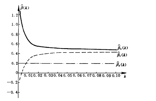I can see it.$k$And the increase, the coefficient is nearing the level of stability, and we're going to have to broadly select the points that have just reached the level of stability as our estimate, because at this point we can try to balance the level of stability with the RSS.

Control the balance squared

The RSS will follow.$k$We choose a constant.$c$ Control Ridge regression factor satisfied $RSS(k)<cRSS(LS)$

Control spread factor

It's the same as the gradual return. We're testing whether or not we're continuing to recoherent.

Hoerl-Kennard Formula

$$\dot{\hat{k}}=\frac{(p-1)\hat{\sigma}^{2}}{\sum_{i=1}^{p}(\hat{\beta}_{i}^{*})^{2}}$$ of which$p$ is the number of variables participating in the return The rest of the variables are estimates of the return of the LS.

LASSO returns.

Summary of models

Least Absolute Security and Shrinkage Advisor
Minimal absolute value enrichment and algorithm regression Adding an estimated optimization function in Ridge$L2$Under the positive influence, Lasso estimates that it's coming.$L1$As punishment. $$\operatorname*{minimize}_{}|y-X\beta|_2^2+\lambda|\beta|_1$$ For LASSO's return due to the addition$L1$It's complicated to continue to work on the analysis.

The LASSO model is characterised by a thin model, which quickly compresses some parameters to zero, and leaves him out of our regression model. In fact, LASSO has played a very powerful role in character selection, and if there's a strong correlation between characteristics, LASSO would prefer to choose one of them and reduce the others to zero. So LASSO is better suited to the small correlation between the features, but the problem of the large number of features.

Superparameter Determination

LASSO's super-parameters are a little more complicated than Ridge's, because we've got a problem with the compression of the number of features, and we've got to combine the two figures below. 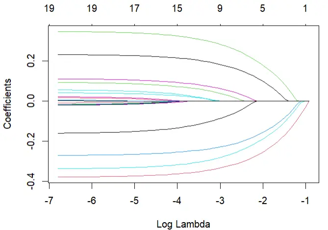This diagram shows how the variables are selected.$log(\lambda)$ It shows the amount left of the signature at this time. 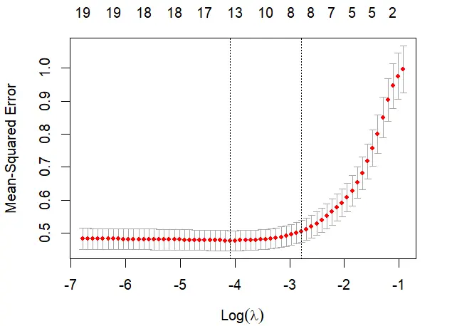This is a map of MSE's involvement.$log(\lambda)$ A combination of MSE and variable compression is what we need to do. We actually have to cross-check the machine learning field to determine the end.$\lambda$ Using a few discounts to cross-check a normal computer will help us decide. Finally we get a minimum MSE.$\lambda$ I can get it.$\lambda$ Your own standard error. If MSE doesn't guarantee a better compression, then a standard wrong scaling will work.

ElasticNet returns

Flex-net regression

Summary of models

So ElasticNet was quickly studied by mathematicians and made the following corrections to the optimisation function, and at this point we need to determine two super-parameters. $$\min Q(\beta)=|y-X\beta|^2+\lambda\alpha\sum_{j=0}^n|\beta_j|+\lambda(1-\alpha)\sum_{j=0}^n\beta_j^2\color{red}$$ ElasticNet was created to combine the strengths of LASSO and Ridge. By combining the L1, L2 model, ElasticNet preserves both LASSO ' s easy-to-resort characteristics and L2 ' s retrogressive nature, while also addressing the problem of LASSO ' s method producing multiple decompositions when multiple variables are highly relevant, effectively removing irrelevant variables from the selection of variables and retaining relevant variables of high relevance.

Superparameter Determination

ElasticNet models need to identify two super-parameters at the same time, but our core thinking hasn't changed. For just making sure$\lambda$ We've already described the treatment in LASSO, which means K-turn cross-check to find MSE. Then add the variable.$\alpha$What's the situation? First select 0.01 to 0.99. $\alpha$ Mixed superparameters I'm sure.$\alpha$ Under the circumstances, we can still use the K-turn cross-check to find the right place.$\lambda$ (minimal MSE) and corresponding standard errors We can match every one of them.$\alpha$The MSE down there found the smallest MSE. That's two super-parameter choices. In fact, in R languages, ElasticNet LASSO uses glment packages for processing. They're doing exactly the same thing. In fact, this is in the assigned parameter domain.$[0,1]$Just re-state the process here.