Linear Time Series Analysis: Stationarity, ARMA, and ARIMA

This English version was machine-translated from the Chinese original. Technical terms may require verification.

Introduction and some basic concepts

Basic definitions

Time series is a series of time points that can be arranged in an orderly fashion.

The data from observation of a series of time points is very common in research, so time series analysis is used in a wide variety of ways.

The research objectives of time series analysis are twofold.

• Study of the mechanisms for the generation of time series Get to know the past.
• Forecasting future possibilities based on historical data and other relevant factors Forecasting the future

In order to achieve time series analysis, we often need to require that time series exist in some built-in structure, and if he is completely random, we often lack the need to study time series.

An example of a time series

Here's a time series. 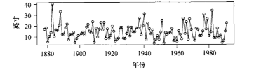It contains a time (which may be the year, the hour, etc.) as a cross-reference, an observation value as a vertical coordinate, and this is the most basic graphic of the time series.

Another common time series chart 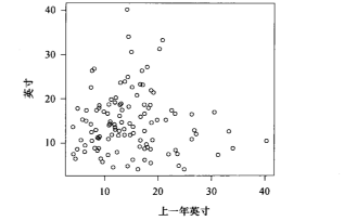It uses the data of the previous year as cross-references, the data of the current year as vertical coordinates, which allows us to study whether there is some influence between the two-year observations.

Time series analysis requires more of our research maps than other areas, and we need to map them against the research targets, and the information in the analysis maps is important to develop an understanding of the charts, and we often choose the appropriate time series analysis model based on the information that the maps react to.

Linear regression and time series analysis

The time series cannot be equated to regression analysis.

The characteristics of the time series data are:

• Self-relevance (linear or non-linear)
• Non-exchangeability (samples sequence is not interchangeable)

The simplest data structure in the application scene of regression analysis is interchangeable.Data for independent and distributedWhen time series data meet some conditions, you can use regression analysis to handle it.$AR$But we can't think of them as identical.

There are a lot of unique ways to do time series analysis, and they have no connection with regression analysis, so...The time series cannot be equated to regression analysis.

Random process and time series analysis

Time series is a set of observations from random processes: We call it the time series process of the random process.

The time series process is a special random process.

Digital features of time series

More commonly used as follows: Mean function defined as $$\mu_{t}=E(Yt)$$ Self-conciliation difference function defined as $$Cov(X_s,X_t)=\operatorname{E}\left[(X_s-m_X(s))(X_t-m_X(t))\right]$$ The function is defined as $$rt s, =mathrm{Corr} (Y t}, Y Y mathrm{Cov} (Y t}, Y s} }{\sqrt{\mathrm{Var} (Y t}\mathrm{Var} (Y}){s})}}=\frac{\gamma{t,s}}{\sqrt{\gamma_{t,t}\gamma_{s,s}}}$$ 他们有一些基础的性质为 $$\begin{aligned}\gamma_{\iota.\iota}&=\operatorname{Var}(Y_{\iota})&\rho_{\iota.\iota}&=1\\gamma_{t.s}&=\gamma_{s.t}&\rho_{t,s}&=\rho_{s,t}\\mid\gamma_{\iota,s}|&\leqslant\sqrt{\gamma_{\iota.t}\gamma_{s,s}}&\mid\rho_{t.s}\mid\leqslant1\end{aligned}$$ 我们这里给出一个有用的定理 $$\mathrm{Cov}\bigg[\sum_{i=1}^{m}c_{i}Y_{t_{i}},\sum_{j=1}^{n}d_{j}Y_{s_{j}}\bigg]=\sum_{i=1}^{m}\sum_{j=1}^{n}c_{i}d_{j}\mathrm{Cov}(Y_{t_{i}},Y_{s_{j}})$$

Let's just go over the concept of random process smoothness here. Random Process Basis “Definition of smooth process” section

Disaggregation of time series

The time series needs an internal structure to be analysed. $$X_t=T_t+S_t+R_t,t=1,2,\ldots $$

• Trends
• Seasonal item
• Random Item We have a lot of natural ideas about how to estimate these items, like using retrogressive convergence trends, and the rest of the items using quarterly average catch seasons, and so on, we'll have a detailed study later on.

Trends and seasons can be treated as non-random time series, and their prediction problems are often simple. Random items are usually smooth sequences.

Examples of common time series

I'm just gonna swim around.

You!$e_1,e_2,...$The difference is$\sigma^2$I'm sorry. I'm looking at the time series of independent and distributed random variables. ${Y_t:t=$ $1,:2,:...}$ Construct as follows: $$\left.\left.\begin array}Y 1&=e_1\Y_2&=e_1+e_2\&\vdots\Y_t&=e 1+e 2+\cdots+e t\end{array}\right.\right}$$ We can easily calculate it. Mean Functions$\mu_{t}=0$ Difference Functions $\mathrm{Var}(Y_{\imath})=t\sigma_{e}^{2}$ Custom Related Functions $\rho_{t,s}=\frac{\gamma_{t,s}}{\sqrt{\gamma_{t,t}\gamma_{s,s}}}={\sqrt{\frac{t}{s}}}$

And we can give you some understanding of randomly moving processes.

Over time, in the next few minutes. Go, go, go!$Y$The value is becoming more relevant, and on the other hand, the time is far away.$Y$Values, which are becoming less relevant, and ac-frograms of the unit root process, which are slow and slow to decline.

Although the theoretical average is zero, the difference increases over time, so the process is expected to swing away from zero, which also shows that the model is unpredictable.

Slide Average

Or the assumptions that lie ahead? $$Y_t=\frac{e_t+e_{t-1}}2$$ Mean Functions$\mu_{t}=0$ Difference Functions $\mathrm{Var}(Y_{\imath})=0.5\sigma_{e}^{2}$ Custom Related Functions $US$US$US$$US$$US$$US$US$US$$US$US$$US$US$$US$$US$US$US$$US$US$US$US$US$$US$US$US$$US$US$US$US$US$$US$US$US$US$US$US$US$US$US$US$US$US$US$US$US$US$US$US$US$US$US$US$US$US$US$US$US$US$US$US$&\mid t-s\mid=0\0.5&\mid t-s\mid=1\0&\mid t-s\mid>You're not gonna get away with this? The average process is a smooth process that is usually used as an example of introduction.

White Noise

An important example of this smoothing is the so-called white noise process, defined as the series of random variables in the same distribution.$\langle e_i\rangle$It's not because it's interesting, but because many useful processes can be constructed by white noise processes.

For white noise processes, there are $E[e_t]=\mu$ $cov(e_t,e_s)=\begin{cases}\sigma^2&t=s\0&I'm sorry, I'm sorry, but I'm sorry, but I'm sorry, but I'm sorry, but I'm sorry, but I'm sorry. If random variables are independent of each other, it's called independent white noise. If the average is 0, then it's called the zero-average independent white noise, and then if the difference is 1 it's called the standard independent white noise.

We usually study the most general standard of independent white noise. We can see that randomly moving and sliding are constructed on average according to white noise processes.

Random Cosine Wave

$$Y_{t}=\cos\left[2\pi(\frac{t}{12}+\Phi)\right]$$ of which $\Phi\sim U(0,1)$ And we can see that this random process has a strong degree of certainty, and it's cyclical, and his only randomity is how we pick and choose our first date. We can figure it out. Mean Functions $\mu_{t}=0$ Custom Related Functions $\rho_k=\cos(2\pi\frac k{12})$ So, we can judge it as a smooth time series. The simulator of the average and random cosine wave of observation shows that it is unrealistic to judge the stability of the time series by relying on our observation time series alone, and we need to find other ways to process it later.

Stable differences

We know that random migration sequences are not stable. But we're not alone. $Y_t$It's about his differences, which is... $$Z_t=Y_t-Y_{t-1}$$ It's easy to see that the sequence after the differential is flat. So we can use the simple technique of differentials to get statistically stable sequences that were not stable.

Trends

This is some of the explanations for the section on the breakdown of time series, which explains the meaning of the trend item.

Trends of certainty and randomity

Trends are the product of observations of reality, but we know that time series are random and that the trends we see are not necessarily the true characteristics of the sequence, so we need to model them over time and find real information from multiple surface trends.

• Random trends: multiple simulations show completely different trends in time series
• Trends of certainty: trends in multiple simulations show near time series

It's very obvious:If we only have one chance to observe, there is no way to judge whether the trend is random or definitive, and we will determine sexual trends in the later studies.

Constant mean

As a simple case, it's also called a smooth time series, so we assume that the average function is constant. $$Y_t=\mu+X_t$$ Random disturbance of which$X_t$Yes.$EX=0$ We can estimate the average value below without adding any other assumptions. $$\overline{Y}=\mu$$ To study the accuracy of this estimate, we need to be right.$X_t$And there's not much to be done here.

Very equal

We need to look at the uneven sequences and make a series of assumptions about changes in the averages to be specific to the analysis.

Linear trends

Consider $$\mu_t=\beta_0+\beta_1t$$ To estimate this situation, we need the minimum two-fold method most commonly used in regression analysis.

Seasonal trends

It's our basic model. $$Y_t=\mu_t+X_t$$ The idea of a more common seasonal model is to follow the monthly pattern. $US$US$US$US$US$US$US$US$US$US$US$US$US$US$US$US$US$US$US$US$US$US$US$US$US$US$US$US$US$US$US$US$US$US$US$US$US$US$US$US$US$US$US$US$US$US$US$US$US$US$US$US$US$US$USE&t=1,13,25,\cdots\\beta_2&t=2,14,26,\cdots\\vdots\\beta_{12}&t= 12, 24, 36, \cdots\end{cases} The estimates of this trend are based on experience and some of the statistical methods that we have not been able to address, and the use of statistical software is needed, and we know that it is enough to analyse them.

Cosine trend

The seasonal average model contains many separate parameters, but it does not take into account the shape of seasonal trends, and only a few time series models are not relevant when they are close, so we introduced cosine trend models, which are very common when they exist. Consider the average model below $$\mu_{t}=\beta\mathrm{cos}(2\pi ft+\Phi)$$

We can deform it below, and we can use regression to deal with it. $$\mu_{t}=\beta_{0}+\beta_{1}\cos(2\pi ft)+\beta_{2}\sin(2\pi ft)$$

Steady Random Time Series ARMA

We're talking about the basic concept of a large class of parameter time series models, which are retrogressive average models (ARMAs), which play an important role in modelling real processes, and their core characteristics are:Steady.

General linear process

I think...$Y_t$It's the time series we've been observing, and we think...$e_t$is a white noise sequence that is not observed; You can set the mean of this white noise sequence to zero, which means we erase the average information, and in a real model, we can be considered to have lost the average. So the general linear process can be seen as a weighted linear combination of past and present white noise. $$Y_{t}=e_{t}+\psi_{1}e_{t-1}+\psi_{2}e_{t-2}+\cdots $$ On the right is an infinite number, and we will be able to limit it more to the goal we want to study.

Slide Average Process (MA)

One very natural idea is that the impact of the very distant noise can be ignored, so we can transform the general linear process into a process that is very, very, very, very, very, very, very, very, very, very, very, very, very, very, very, very, very, very, very, very, very, very, very, very, very, very, very, very, very, very, very, very, very, very, very, very, very, very, very, very, very, very, very, very, very, very, very, very, very, very, very, very, very, very, very, very, very, very, very, very, very, very, very, very, very, very, very, very, very, very, very, very, very, very, very, very, very, very, very, very, very, very, very, very, very, very, very, very, very, very, very, very, very, very, very, very, very, very, very, very, very, very, very, very, very, very, very, very, very, very, very, very, very, $$Y_t=e_t-\theta_1e_{t+1}-\theta_2e_{t-2}-\cdots-\theta_qe_{t-q}$$ The coefficient is random, the positive. We call it the equation.$q$Slipping average process as$MA(q)$ The slide average is the average based on the weight, then the average is re-enacted at a time, and so on.

MA（1）

Model as $$Y_{t}=e_{t}-\theta e_{t-1}.$$ It's easy to calculate. $$E(Y_{t})=0$$ $$\mathrm{Cov}(Y_t,Y_{t-1})=\mathrm{Cov}(e_t-\theta e_{t-1},e_{t-1}-\theta e_{t-2})=\mathrm{Cov}(-\theta e_{t-1},e_{t-1})=-\theta \sigma_t^2$$ $$\mathrm{Cov}(Y_t,Y_{t-2})=\mathrm{Cov}(e_t-\theta e_{t-1},e_{t-2}-\theta e_{t-3})=0$$ It can be seen that there is no self-relevance after the process is older than level one. We can base our actions on specifics.$\theta$The value is taken to analyse the magnitude of the coefficient, and it can also be analysed for relevance, as we have shown at the beginning of the section on "Sequence-Sequence Examples"

MA（2）

Model as $$Y_{t}=e_{t}-\theta_{1}e_{t-1}-\theta_{2}e_{t-2}$$ Compute the synergetic difference function has $$\gamma_0=\mathrm{Var}(Y_t)=\mathrm{Var}(e_t-\theta_1e_{t-1}-\theta_2e_{t-2})=(1+\theta_1^2+\theta_2^2)\sigma_{t}^{2}$$ $$\begin{aligned} \gamma_{1}& =\mathrm{Cov}(Y_{i},Y_{i-1})=\mathrm{Cov}(e_{i}-\theta_{1}e_{i-1}-\theta_{2}e_{i-2},e_{i-1}-\theta_{1}e_{i-2}-\theta_{2}e_{i-3}) \ &=\mathrm{Cov}(-\theta_1e_{t-1},e_{t-1})+\mathrm{Cov}(-\theta_1e_{t-2},-\theta_2e_{t-2}) \ &=[-\theta_1+(-\theta_1)(-\theta_2)]\sigma_e^2=(-\theta_1+\theta_1\theta_2)\sigma_e^2 \end{aligned}$$ $$\begin{gathered} \gamma 2} == sync, corrected by elderman == I'm sorry, I'm sorry. That's right.$MA(2)$ Models larger than second tier lags are not self-relevant

MA（q）

We'll give you a direct conclusion on the function. $US$\rho k=begin{cases}\fra{k+theta k+theta \theta \ \q^}&\quad k=1,2,\cdots,q\0&\quad k>q\end{cases} The conclusion is clear. $MA(q)$Process is greater than$q$There's no correlation when you're lagging behind. We've done enough research on the average slide process. We'll go on to another important model.

Self-Return Process (AR)

By definition, self-return refers to self-returning as a regression variable. This is in the form of:$p$Step-by-step process meets equations $$Y_t=\phi_1Y_{t-1}+\phi_2Y_{t-2}+\cdotp\cdotp\cdotp+\phi_pY_{t-p}+e_t$$ That's right.$p$A lag item and new message entry$e_t$

AR（1）

Or do you start with a simple form? $$Y_{t}=\phi Y_{t-1}+e_{t}$$ We'll assume the average is zero, and it'll be on a smooth condition. Let's calculate. $$\gamma_0=\frac{\sigma_e^2}{1-\phi^2}$$ $$\gamma_k=\phi^k\frac{\sigma_e^2}{1-\phi^2}$$ $$\rho_k=\frac{\gamma_k}{\gamma_0}=\phi^k$$ Because the difference must be right, $1<\phi<$1. So we know that the function of the function in question is characterized by an index decrease, and that, depending on the positive and negative, it's a serene type. We might as well take it.$\phi=0.9$ It can be seen that even a third-level lag has a strong self-relevance. We can easily prove it.<\phi<1$ 的时候 $AR(1) process is smooth.

AR（2）

Model in the form of $$Y_t=\phi_1Y_{t-1}+\phi_2Y_{t-2}+e_t$$ To make the model stable, we need to meet the conditions. $ \phi 1+\phi 2<1,\quad\phi_2-\phi_1<1\text{,}\quad|\phi_2|<1$$ 为了研究自相关函数 我们沿用上面的思路得到下面的递推方程 Yule-Walker 方程 $$\rho_{k}=\phi_{1}\rho_{k-1}+\phi_{2}\rho_{k-2},\quad k=1,2,3,\cdotp\cdotp\cdotp $$ 其中为了进行递推有 $$\rho_1=\frac{\phi_1}{1-\phi_2}$$ $$\rho 2 = \ \ \ \ \ \ \ \ \ \ \ \ \ \ } } } } } } } } } } } } } } } } = = = = = $ $ $ $ $ $ $ $ \ $ $ $ $ $ $ \ \ $ $ $ $ \ \ \ \ \ \ \ \ \ \ \ \ \ \ \ \ \ \ \ \ \ \ \ \ \ \ \ \ \ \ \ \ \ \ \ \ \ \ \ \ \ \ \ \ \ \ \ \ \ $ $ $ \ \ \ \ \ \ \ \ \ \ \ \ \ \ \ \ We study the incremental formula of the function to analyse the nature of the function, and positive or negative changes are possible as the lag step increases from the index of the relevant coefficient. This decline could be index decline or block the nymphosphate.

AR（p）

Consider the model as $$Y_t=\phi_1Y_{t-1}+\phi_2Y_{t-2}+\cdotp\cdotp\cdotp+\phi_pY_{t-p}+e_t$$ And give the necessary conditions for stability: $$\begin{aligned}\phi 1+\phi 2+\cdots+\pi p<1\|\phi_p|<1\end{aligned}$$ 给出Yule-Walker方程为 $$\begin{aligned}\rho_1&=\phi_1+\phi_2\rho_1+\phi_3\rho_2+\cdots+\phi_p\rho_{p-1}\\rho_2&=\phi_1\rho_1+\phi_2+\phi_3\rho_1+\cdots+\phi_{p,p-2}\&\vdots\\rho_p&=cdots+\ft p\d{aligned} I'm sorry. If we give a specific coefficient, we can solve the coefficients by the equation. The nature of the relevant coefficients is:The coefficient is a linear combination of some resistance to nectar and some resistance to swirl fluctuations.

Average Slipper Process (ARMA) for self-return

If one of the models is self-regressive, the other is sliding average, there's a more general model form (or flat) $$Y_t=\phi_1Y_{t-1}+\phi_2Y_{t-2}+\cdots+\phi_pY_{t-p}+e_t-\theta_1e_{t-1}-\theta_2e_{t-2}-\cdots-\theta_qe_{t-q}$$ We call it$ARMA(p,q)$ We'll just introduce a simple form.

ARMA（1）

Model defined $$Y_t=\phi Y_{t-1}+e_t-\theta e_{t-1}$$ Because of the presence$AR$The ingredients, we need to consider the condition of stability. $$\mid\pi\mid<1$$ 通过一系列运算有 自相关函数为 $$\rho k=\frac(1-\theta\i) (\theta)\1-2\theta\pi+\theta^)\rho=,\fad k\geqslant$1 He's also a form of index decline.$p_0$ (Dependantly)$\theta$) This is the one that makes it$AR(1),MA(1)$ It's different. One of them is a step behind.$\theta$ The other one is index decline but starting with 1.

For the general ARMA model, we're meeting the level of stability. $$\text{当月仅当 AR 特征方程 }\phi(x)=0\text{ 的根的模大于 }1$$ Satisfactory to the relevant function at this time $rho k=k 1}k=k\k\k\>q$ A form similar to the Yule-Walker equation when $k<q$的时候 自相关函数会含有$\theta$ ingredients

Reversibility

We can actually see it in front of us.$MA$Models. We use them.$MA(1)$ For example, $$\mathrm{Cov}(Y_t,Y_{t-1})=\mathrm{Cov}(e_t-\theta e_{t-1},e_{t-1}-\theta e_{t-2})=\mathrm{Cov}(-\theta e_{t-1},e_{t-1})=-\theta \sigma_t^2$$ And then there was... $$\rho_{1}=(-\theta)/(1+\theta^{2})$$ It's easy to find.$\theta,\frac{1}{\theta}$ The relevant coefficients are the same.

And even if we take the value of a known correlation coefficient, the coefficients that we get are not the only ones that are the same.

We know that the AR process can be described as a general linear process. What about the MA process? We'll think about it. $$Y_t=e_t-\theta e_{t-1}$$ Convert $$e_{t}=Y_{t}+\theta e_{t-1}$$ And then they keep changing.$e_{t-1}$ Yes. $$e_t=Y_t+\theta Y_{t-1}+\theta^2Y_{t-2}+\cdotp\cdotp\cdotp $$ So there is. $$Y_t=(-\theta Y_{t-1}-\theta^2Y_{t-2}-\theta^3Y_{t-3}-\cdots)+e_t$$ Which means if we have a t-shirt,<1$ 则$MA(1)$ 可以转化为一个自回归模型 此时我们称其为可逆的$MA$ Model For the general$MA,ARMA$ Models, they can reverse if the root of the characteristic equation is more than one. We can easily prove:For reversible MA processes, a single set of parameters can be obtained in the case of a given function We're working on it.$ARMA$Models are both smooth and reversible.

Unstable Random Time Series ARIMA

Not all event sequence models are stable; in fact, most time series models in the real world are non-stable, and the forced use of the method modelling in the "Stable and Random Time Series ARMA" section of this paper can only produce absurd conclusions.

Fortunately, we need only a simple way to study the problem of instability.

AR model involves smoothing (factors) MA model involves reversible issues (or is it related to coefficients) And then the ARMA model, the ARIMA model, will study them at the same time.

Stable differences

Let's think about one.$AR(1)$ Model $$Y_t=3Y_{t-1}+e_t$$ This doesn't fit the description.$AR(1)$ The conditions for stabilization studied by the model Actually... $$\mathrm{Var}(Y_{t})=\frac{1}{8}(9^{t}-1)\sigma_{e}^{2}$$ The difference has an exponential explosion. $$\mathrm{Corr}(Y_{t},Y_{t-k})=3^{k}\sqrt{\frac{9^{t-k}-1}{9^{t}-1}}\approx1.$$ For the larger$t$ And medium strength.$k$ The index explosion is the cause of this correlation. And that's that, in any case, this time series will be exponential.

We'll think about it. $$Y_t=Y_{t-1}+e_t$$ Compute its first-class differential. $$\nabla Y_t=e_t$$ It's easy to see that the difference can stabilize the original unstable model. The phenomena described above are widespread, the differentials are conducive to smoothing the unstable model, and if the first step is not enough, then the difference is empirically enough.

ARIMA Model

If a time series model${Y_t}$ Yes.$d$The sub-division is a flat ARMA model, which is called an ARIMA model if the differential obeys$ARMA(p,d)$ Name $Y_t$ Obey.$ARIMA(p,d,q)$ Think about one next.$ARIMA(p,1,q)$ You!$W_t=Y_t-Y_{t-1}$ $$W_t=\phi_1W_{t-1}+\phi_2W_{t-2}+\cdots+\phi_pW_{t-p}+e_t-\theta_1e_{t-1}-\theta_2e_{t-2}-\cdots-\theta_qe_{t-q}$$ Or as an expression $$00\&\phi_1(Y_{t-1}-Y_{t-2})+\phi_2(Y_{t-2}-Y_{t-3})+\cdots+\phi_p(Y_{t-p}-Y_{t-p-1})\&+e_t-\theta_1e_{t-1}-\theta_2e_{t-2}-\cdots-\theta_qe_{t-q}\end{aligned}$$ 可以改写为 $$\begin{aligned}Y_t&=(1+\phi_1)Y_{t-1}+(\phi_2-\phi_1)Y_{t-2}+(\phi_3-\phi_2)Y_{t-3}+\cdots\&+ (\p-\ph) Y t-p}- \\ph p t-p e t-\theta 1e t t \theta 2 t}-\cdots-\theta qe {t-q} I'm sorry. To understand these three forms The first one is one.$ARMA(p,q)$ The second is just a change of name, and the third is a change of name. $ARMA(p+1,q)$

IMA(1,1)

We're still thinking about the simplest form. $$Y_{t}=Y_{t-1}+e_{t}-\theta e_{t-1}$$ The differences and related factors in calculating the model are: $$\left.\mathrm{Var}(Y_{i})=\left[\begin{matrix}{1+\theta^{2}+(1-\theta)^{2}(t+m)}\\end{matrix}\right.\right]\sigma_{\epsilon}^{2}$$ Showing explosion. $$00\ \\mathrm{Corr} (Y ({\ota}, Y t-k}& =\frac{1-\theta+\theta^2+(1-\theta)^2(t+m-k)}{[\operatorname{Var}(Y_t)\operatorname{Var}(Y_{t-k})]^{1/2}}\approx\sqrt{\frac{t+m-k}{t+m}} \ &\\approx1 I'm sorry, I'm sorry. The reason for the explosion is the strong correlation.

IMA(2,2)

Model as $$\nabla^2Y_t=e_t-\theta_1e_{t-1}-\theta_2e_{t-2}$$ We do not calculate, answer directly, and the difference and the related coefficients are presented in the same way as in this paper, "IMA (1, 1)." Section

Constants in ARIMA

In the section on "Arma for a smooth, random time series" here, constants are not affecting our research, less averages, and zero values are studied, and all results plus averages are sufficient. But in ARIMA, it's not that simple. It's easy to introduce the model into the differential model, as follows: $$00\ W t}-mu=& \phi_{1}(W_{t-1}-\mu)+\phi_{2}(W_{t-2}-\mu)+\cdots+\phi_{p}(W_{t-p}-\mu) \ &+e_{t}-\theta_{1}e_{t-1}-\theta_{2}e_{t-2}-\cdots-\theta_{q}e_{t-q} \end{aligned}$$ 或者 $$W_t=\theta_0+\phi_1W_{t-1}+\phi_2W_{t-2}+\cdots+\phi_pW_{t-p}+e_t-\theta_1e_{t-1}-\theta_2e_{t-2}-\cdots-\theta_qe_{t-q}$$ 其中 $$Other Organiser They're actually equal.

We need to consider the impact of this non-0-average on the original ARIA model. IMA (1,1).$Y_t$Yes. $ \begin{aligned}Y t=&e_t+(1-\theta)e_{t-1}+(1-\theta)e_{t-2}+\cdots+(1-\theta)e_{-m}-\theta e_{-m-1}\&+ (t+m+1)\theta The fact that the IMA is not a zero average has led to a linear trend over time. Yes.$d=2$ Time Non-0-average leads to a double time trend item

Data transformation in time series analysis

In many realities, we're going to show a percentage increase, especially in economic and biological data, which is actually an exponential growth in time series.

We're doing a logarithmic variant that works very well at this point, and a very important shift in numbers. Group

BoxCox certainly is not just for regression analysis and variance analysis, but there are many things that help us to choose specifics.$\lambda$The way they do it, they usually study normality and variance.

Data conversion is also a very common operation in data analysis, not binding on TSA, and when we choose to change and not study it, as a mere reminder:The time series of data changes are also a very useful technique.

Model recognition

We have developed a large array of time series models, ARIMA; now we have to learn to do statistical extrapolation from the research we have done before, and our work is divided into four parts.

• Select the appropriate time series data for the given time series$p,d,q$Value
• Parameters for estimating the selected model
• Test the proposed model and make improvements
• Forecast future data using previously identified models So that's model recognition, parameter estimates, model tests, model predictions, four parts, and we'll be talking about these in four chapters, including this chapter.

Identification of MA models

We can estimate that the sample has its own function. $$r_{k}=\frac{\sum_{t=k+1}^{n}\left(Y_{t}-\overline{Y}\right)\left(Y_{t-k}-\overline{Y}\right)}{\sum_{t=1}^{n}\left(Y_{t}-\overline{Y}\right)^{2}},\quad k=1,2\cdots $$ Our purpose is to identify the samples from their own relevant functions. Out$r_k$The pattern of the ARIMA model, which is already known, is the appropriate model to be selected.$p,d,q$

Yes.$MA(q)$ Model when the lag step exceeds$q$. This means that the sample is already the relevant function.$MA$A good indicator of the process.

Use sample ACF to identify

Identification of AR Models

But, yes,$AR(p)$Models are becoming progressively decaying from the function in question.$AR(p)$ Model We introduce. $k$The relevant function of the step lag is $$\begin{aligned}\phi_{kk}=\mathrm{Corr}(Y_t-\beta_1Y_{t-1}-\beta_2Y_{t-2}-\cdots-\beta_{k-1}Y_{t-k+1},\Y_{t-k}-\beta_1Y_{t-k+1}-\beta_2Y_{t-k+2}-\cdots-\beta_{k-1}Y_{t-1})\end{aligned}$$ The following is the calculation of the selected function of the sample. $$\phi_{kk}=\frac{\rho_k-\sum_{j=1}^{k-1}\phi_{k-1,j}\rho_{k-j}}{1-\sum_{j=1}^{k-1}\phi_{k-1,j}\rho_j}.$$ What are the characteristics of the function? Yes.$AR(p)$Model $US$ k=,\dk=>P$ That's right. $AR(p)$ Models are given preference from the good indicator of the function $MA(q)$The model has no indication of preference for the function. He'll index decay instead of zero.

Use sample PACF to identify

Identification of ARMA models

ARMA(p,q) does not have a tailing nature for either indicator function We need to come up with new ways to achieve this, and there is more than one way we've put forward to solve the problem of the ARAMA model, and we've introduced the EACF method, which is currently being simulated as being of a more positive nature.

The core idea of the EACF law is:If the AR of a model is known, the observation sequence filtering out of the regression section will get a pure MA model that can be used to determine the order of magnitudes by ACF.

Consider$ARMA(1,1)$To describe the use of the EACF. $$Y_t=\phi Y_{t-1}+e_t-\theta e_{t-1}$$ In this case, apply$Y_t$Yeah.$Y_{t-1}$ Simple linear regression is possible.$\phi$Unsatisfactory estimates (systematic deviations because the quantity of regression factor estimates by nature contains$\theta$But this re-entry is a real disability that can help us analyze. Second Re-entry$Y_t$ The coefficient of return for the first step of the first degree of disability$\tilde{\phi}$ Yeah.$\phi$The same estimate, that is, $$W_{t}=Y_{t}-\tilde{\phi}Y_{t-1}$$It's one.$MA(1)$Process

For ARMA models, it's a good way to think about EACF and the corresponding zero-point point. 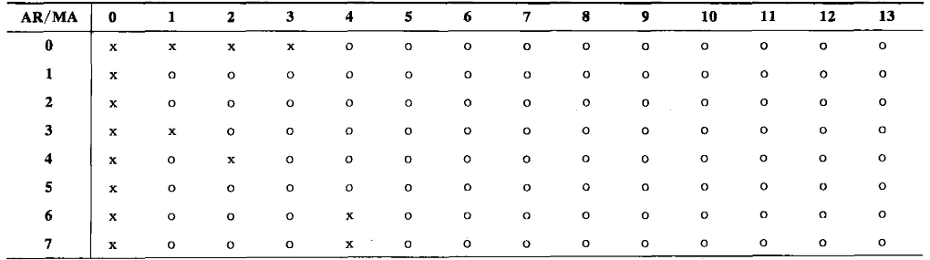Consider the zero triangle.$MA(1),AR(1or2)$ It's all acceptable.

ARIMA Model recognition

The idea of recognition of models

We present here in the section “ARIMA of the non-stable random time series” the unstableness that can be explained by the ARIMA model; All ACF calculations using unstable sequences do not mean anything (ACF calculations are themselves assumed to be smooth)

But we have found nature in a lot of research:The ACF of the non-stable sequence shows a slow downward trend in non-indexed decline

This is not even a ma ARMA model, which can be considered a good way to judge the Alima model.

After judging the ARIMA model, the difference is our only choice.

About the excess differential

We've been talking about the ARIMA section of the non-stable random time series, and the difference in the smooth sequence is still flat; but the excess is not desirable.

When we do the difference, we need to estimate it once more.$\theta$Values, he's also seriously affecting the parameters.

Models should be built as concisely as possible, and excessive differentials are not desirable, but we must also be decisive in the absence of a clear margin.

Other model identification methods

We have a lot of pure-value-based methods. Dickey - Fuller Root Check Select the best model using information volume guidelines such as AIC BIC

Parameter estimation

We've solved the problem of modeling.$p,d,q$ Now we've identified the parameters in the model, and we've only been able to consider the ARMA model, and then the ARMA model, and then the ARMA model, which is not the average, is reduced to their average.

Rectangular estimate

The rectangular estimate is not considered the most efficient method, but it's the simplest way, or the sampler is the theoretical rectangular method, and it's made up of equations that can be estimated by any unknown parameter, the most classic example of which is the estimate of the overall average by the sample average.

Self-Regression Model AR

Yes.$AR(1)$We have models. $$\rho_{1}=\phi.$$ So we calculate the sample from its own function.$r_k$Yes. $r_1=\phi$ Yes.$AR(2)$Model $$r_1=\phi_1+r_1\phi_2,\quad r_2=r_1\phi_1+\phi_2$$ Higher$AR$The model is the same thing.

Slide Average Model MA

For the slide average model, rectangular estimation is not very good.$MA(1)$Yes. $$\rho_1=-\frac\theta{1+\theta^2}$$ We'll take over.$r_1$ We're dealing with a double equation. $$\hat{\theta}=\frac{-1+\sqrt{1-4r_1^2}}{2r_1}$$ This is at $US$US$US$US$US$US$US$US$US$US$US$US$US$US$US$US$US$US$US$US$US$US$US$US$US$US$US$US$US$US$US$US$US$US$US$US$US$US$US$US$US$US$US$US$US$US$US$US$US$US$US$US$US$US$US$US$US$US$US$US$US$US$US$US$US$$US$US$US$US$US$US$US$US$US$US$US$US$US$US$US$US$US$US$US$US$US$US$US$US$US$US$US$$US$$US$US$US$$US$US$$$$$$$US$$$$$$$$$$$$$$$$$$$$$$$$$<If you can solve it with 0.5 dollars, otherwise there's no real solution to this equation; For higher-grade MMA models, it's rapidly becoming more complex.

ARMA

We'll think about it.$ARMA(1,1)$Situation $$\hat{\phi}=\frac{r_{2}}{r_{1}}$$ $$r_1=\frac{(1-\theta\hat{\phi})(\hat{\phi}-\theta)}{1-2\theta\hat{\phi}+\theta^2}$$ We still need to deal with a secondary equation that is more problematic when it exists.

Noise difference

The last amount we need to estimate is the noise. Bad$\sigma_e^2$ First we know we can estimate the sequences with sample differences. Bad $$s^{2}=\frac{1}{n-1}\sum_{\iota=1}^{n}{(Y_{t}-\overline{Y})^{2}}$$ And then we use the text of the difference that was presented in the smooth model to estimate the noise. Bad $AR(p)$ $$\hat{\sigma}{e}^{2}=(1-\hat{\phi}{1}r_{1}-\hat{\phi}{2}r{2}-\cdots-\hat{\phi}{p}r{p})s^{2}$$ $MA(q)$ $$\hat{\sigma}{\epsilon}^{2}=\frac{s^{2}}{1+\hat{\theta}{1}^{2}+\hat{\theta}{2}^{2}+\cdots+\hat{\theta}{q}^{2}}$$ $ARMA(1,1)$ $$\hat{\sigma}_e^2=\frac{1-\hat{\phi}^2}{1-2\hat{\phi}\hat{\theta}+\hat{\theta}^2}s^2$$

Summary

Based on the results of the previous calculations, we can easily draw the following conclusions.

• The rectangular estimates of the self-regression model are acceptable.
• It's hard to get a rectangular estimate of sliding the average model.
• The results of the rectangular estimates of the hybrid model are unacceptable.
• The MA component causes the result of the rectangular estimation to be very poor.

Minimal 2x10 estimate

And at this point, we're introducing an average in the flat model.$\mu$ From that point on, the lowest two-fold estimate is a good way to estimate it.

Self-Regression Model AR

Consider$AR(1)$Situation $$Y_t-\mu=\phi(Y_{t-1}-\mu)+e_t$$ We can see it.$Y_t$Cause variable $Y_{t-1}$ As a regression model for the variable, the lowest quadrilateral study is the minimization of the deviation squared, which is $$S_{\epsilon}(\phi,\mu)=\sum_{\iota=2}^{\pi}\bigl[(Y_{\iota}-\mu)-\phi(Y_{t-1}-\mu)\bigr]^{2}$$ Minimize Based on the method of calculating the minimum two-fold factor, we can estimate it. $$\mu=\overline{Y}$$ $$\hat{\phi}=\frac{\sum_{t=2}^n{(Y_t-\overline{Y})(Y_{t-1}-\overline{Y})}}{\sum_{t=2}^n{(Y_{t-1}-\overline{Y})^2}}\quad.$$ They're not accurate estimates, but the errors caused by the missing items can be ignored in terms of smoothing the process. We can easily promote these results to higher-level AR models. Medium The results given by the minimum quadrilateral are not very different from those estimated by AR model and rectangular.

Slide Average Model MA

Think of the simplest.$MA(1)$Situation $$Y_t=e_t-\theta e_{t-1}$$ It doesn't look like the least double-drive. But we can give the MA model the nature of a near-regressive model, if reversible, as follows: $$Y_t=-\theta Y_{t-1}-\theta^2Y_{t-2}-\theta^3Y_{t-3}-\cdots+e_t$$ Because of the parameters that need to be addressed$\theta$There's a non-linear presence, so we need to use some numerical solvers. For higher-level situations, it's possible to solve it in an iterative manner.

Mixed Model

Consider$ARMA(1,1)$ $$Y_t=\phi Y_{t-1}+e_t-\theta e_{t-1}$$ We're still considering the squared-out minimization of the difference. $$e_t=Y_t-\phi Y_{t-1}+\theta e_{t-1}$$ At this point, we're involved in selection.$e_i$The initial value, but we can choose freely, and in the case of a large sample, it has little effect on the final outcome.

Very similar estimates.

For the sequences and random season models of the length, the selection of the initial values has a significant impact on the final estimate of the parameters, so we have introduced the best method of estimation -- the MLE.

Appearance Functions$L$Defines the probabilistic density function for obtaining actual observations, which is also considered as the function of unknown parameters of the model when observations are fixed;$ARIMA$Models. After the observations.$L$It's the function of model parameters.

The exact estimation method is omitted here.

Model diagnostics

Now, let's consider the advantages of testing models, analysing the residuals, analysing over-parametric models, and they're also the usual ideas for the retrogressive diagnosis.

Disability analysis

The disability analysis is the most extensive analytical method involved in the synthesis of the problem, and the most basic part of the diagnosis of the entire model. Linear regression base And here we're going to show some of the time series analysis methods. The definition of disability is still the same as before. $$\text{残差}=\text{实际值}-\text{预测值}$$

Time series of disability

An ideal, no pattern of the gap figure should show a rectangular dispersion of the line around zero horizontal lines without trend, as follows: 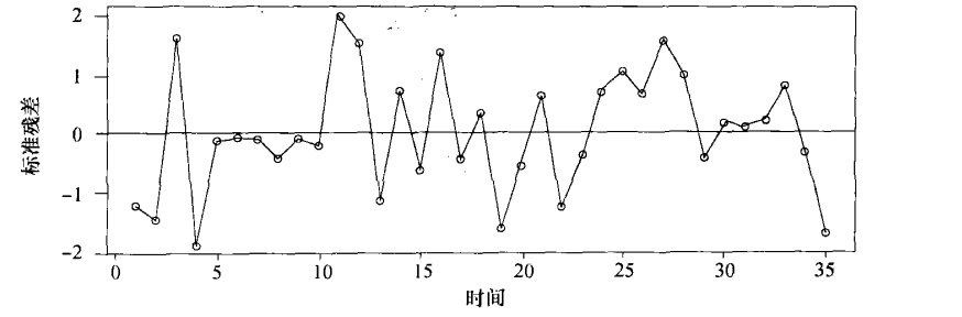This is a basic ideal time series. Figure The time series of the residuals is usually used for the abnormal value test.

Normality test for disability

In the process of modelling, we assumed that the disability had a normal analysis, and that the normality test for the disability was appropriate at this time, and that the more common methods of normality testing were the following:

• QQ Q Chart
• Non-parameter tests such as Shapiro-Wilk Normality Test

Self-relevance of the disability

We were looking at time series models and we were asking that the noise item be independent, and this noise item was shown in the sample as a disability. For real white noise and bigger than that.$n$ (a) The normal distribution of the sample from a function that is almost unrelated and has zero equal value; But even the correct identification model that is effective in estimating the parameters has different characteristics. The normal difference is almost equal to the normal anger distribution of zero.$\frac{1}{n}$ For a large lag, the approximation difference.$\frac{1}{n}$

Intuitive approach

Now we need to look at the specific problem; we can draw the ACF curve of sample differences, and if it's less than the criticality of the gap, then basically the disability is not relevant.

It is particularly important to note that the ACF, which lags behind 4 (quarterly data)12 (monthly data), is likely to exceed the threshold, as we will describe in more detail where the seasonal model is located.

Ljung-Box Test

We studied the self-relevant coefficients of the residuals that are lagging alone, and it's actually interesting to see these factors together.Mathematical statistics and the study in the “Relevance coefficient” section We're putting in statistics. $Q=n{1}^{2}+\hat{r}+\cdots+\hat{r}$$ If the estimate is correct,$ARMA(p,q)$Models, in large sample cases, it's almost submissive.$\chi^2(K-p-q)$

Unfortunately, this conclusion is not good for smaller samples, so Ljung and Box have proposed amendments to the typical sample capacity. $$Q_{\star}=n(n+2)\Big(\frac{\hat{r}_1^2}{n-1}+\frac{\hat{r}_2^2}{n-2}+\cdots+\frac{\hat{r}_k^2}{n-K}\Big)$$ It's better than the statistics above are similar to the calorie distribution.

In practice, we'll reduce the freedom of the parameters according to the number of free parameters and adjust the parameters of the Ljung-Box test.

Overcompatibility and argument redundancy

This is another diagnostic method that is more important in time series analysis; the question we want to end is, in part, like$AR(2)$The model is already working well in small amounts, but we've been over the edge as well.$AR(3)$And this is the time to correct this error. We need to minimize the complexity of models, as conditions permit.

We believe there is an over-compatibility in the following circumstances.

• Additional parameters are not significant or 0
• There is no change in the common parameters compared to the original estimate In part, we'll use model numbers, like AIC values, to aid some of these judgments.

We also have some suggestions at the design stage of the model to avoid overcompatibility.

• Use simple models to the extent possible and, if not, consider reprocessing by means such as disability analysis, if possible
• Do not add the ranks of AR MA I

Model prediction

In fact, predictions are the purpose of the time series modelling, and time series analysis is not at all as coefficients as retrogressive analysis can analyse, so so predictions are made and the accuracy of the predictions is the final part of the whole time series analysis.

Minimal average error forecast

Sequences can be obtained until time$t$The data, that's...$Y_1,...Y_t$ We want to predict the future.$l$The data of the period, that's...$Y_{t+l}$ We call time.$t$As the starting point for projections $l$For predicting step or advance time In some of the certificates we omitted, we concluded that$l$The minimum average error of step is projected $$$$1 }t(\ell)=E(Y|Y 1, Y 2, \\cdotp\cdotp, Y t) $ This is a very important conclusion, and all the projections we take are the smallest MLE projections, and it is expected that this will simplify many of our problems.

Trends in certainty

Here, our certainty trends are not about observations that represent the real situation, but about the mechanisms that are inside our known models. Here's the example of how we can understand the basics of our predictions. Consider $$Y_t=\mu_t+X_t$$ of which$X_t$is the known difference white noise of zero averages $$00\ What's wrong with you?{t}(\ell)& =E(\mu{t+\ell}+X_{t+\ell}|Y_{1},Y_{2},\cdotp\cdotp\cdotp,Y_{\iota}) \ &=E(\mu_{t+\ell}\mid Y_1,Y_2,\cdots,Y_t)+E(X_{t+\ell}\mid Y_1,Y_2,\cdots,Y_t) \ &=\mu_{t+\ell}+E(X_{t+\ell}) \end{aligned}$$ 也就是 $$\hat{Y}{\iota}(\ell)=\mu{\iota+\ell}$$

Projected error is $e t}(\ell)=Y t+ell}-hat{Y}{t}(\ell)=\mu{t+\ell}+X_{t+\ell}-\mu_{t+\ell}=X_{t+\ell}$$ 研究预测误差有 $$E(e_{t}(\ell))=E(X_{t+\ell})=0$$ $$\mathrm{Var}(e t}( \ell)=mathrm{Var} (X t+ell}=gamma $$$) That's what the prediction is, neutral and the difference is fixed.

ARIMA projections

Now we're extrapolating the models from data, then estimating the parameters, and then predicting them, and there's a different way of doing it, and we need to add a few sections of the carrying, and the rest of the narrative will be a whole, and we'll have to look at the whole picture.

AR Model

We're from non-zero averages.$AR(1)$The model begins, and then the natural extension understands the entire AR model. Model form $$Y_{t}-\mu=\phi(Y_{t-1}-\mu)+e_{t}$$ We're gonna make a step-by-step prediction. $$Y_{t+1}-\mu=\phi(Y_t-\mu)+e_{t+1}$$ Based on the minimum MSE projections, we expect to have $$$$1 }{t}(1)-\mu=\phi[E(Y{t}\mid Y_{1},Y_{2},\cdots,Y_{t})-\mu]+E(e_{t+1}\mid Y_{1},Y_{2},\cdots,Y_{t})$$ 根据条件期望的性质我们可以实现化简 $$\hat{Y}{t}(1)=\mu+\phi(Y- You're not gonna get it. I can see that. The first-order AR model is essentially compressed (coefficient absolutes less than 1) and the last model will conceivably reach the average. Wants to predict more steps.OrganisationOur predictions are good.

The prediction error of the model is also very well studied. $$$1=Y={t}(1)=\left[\phi(Y{t}-\mu)+\mu+e_{t+1}\right]-\left[\phi(Y_{t}-\mu)+\mu\right]$$ 也就是 $$e_t(1)=e_{t+1}$$ 一步向前预测误差是AR噪声 我们也可以轻松的给出预测误差的方差（期望为0必然） $$\mathrm{Var}(e_{t}(1))=\sigma_{e}^{2}$$ 研究多步预测的误差有 $$=t(\ell)=e t+t+t\t\t\t\t\t\t\t\psi t t t+t+t+t\cdots+psi e t+t+t+t+t+t+t+ Of which$\psi$It's the form of a coefficient deformation. This form is set for the Alima model. It's easy to judge. $$\mathrm{Var}(e_t(\ell))=\sigma_e^2(1+\psi_1^2+\psi_2^2+\cdotp\cdotp\cdotp+\psi_{\ell-1}^2)$$ This form is also set up for all ARIMA models.

As for the other nature of this value, we're going to come to the conclusion that For all the flat ARMA models, there are... $$\mathrm{Var}(e_{\iota}(\ell))\approx\mathrm{Var}(Y_{\iota})=\gamma_{0},\text{对较大的 }\ell $$ We've come to three conclusions that go beyond the AR model.

MA Model

We're here to consider how to deal with the average slide ingredient.$MA(1)$ Yes. $$Y_t=\mu+e_t-\theta e_{t-1}$$ One step forward, and the conditions are expected to be. $$$$1 }{\iota}(1)=\mu-\theta E(e{t}|Y_{t},Y_{2},\cdots,Y_{t})$$ 然而我们知道（这是一个在$t$较大的时候成立的逼近结论） $$E(e_t\mid Y_1,Y_2,\cdotp\cdotp\cdotp,Y_t)=e_t$$ 因此 一步预测的表达式为 $$\t(1)=mu \theta e t$ Of which$e_t$As a first$t$The difference in the steps was determined when the model was ready.

The MMA model's multistep predictions show some slight changes, as follows: $$$$1 }t(\ell)=\mu+E(e\midY 1, Y 2, \cdotp\cdotp, Y t) \theta e(e t+ell )\midY 1, Y 2, \cdotp\cdotp, Y t) $ We found out we were right over$t$The steps are broken without any knowledge. There's no real value. No disability. But we know. Disabled$e_{t+l}$ and$Y_i$So the condition is zero, so the MMA model's multistep prediction is, $$$$ =m,}}Y >1$$ We don't introduce the M.A.'s prediction error. We'll just follow the three conclusions that AR gave us.

ARMA Model

We're giving the predictions directly in the form of: $ \begin{aligned}i(\ell)&=\phi_1\hat{Y}i(\ell-1)+\phi_2\hat{Y}i(\ell-2)+\cdots+\phi_p\hat{Y}t(\ell-p)+\theta_0-\theta_1E(e{t+t-1}\mid Y_1,Y_2,\cdot\cdot\cdot,Y_t)\&-\theta_2E(e{t+t-2}\mid Y_1,Y_2,\cdot\cdot\cdot,Y_t)-\cdot\cdot\cdot-\theta_eE(e{t+t-q}\mid Y_1,Y_2,\cdot\cdot\cdot,Y_t)\end{aligned}$$ 其中有 $$E(e{t+j}\mid Y_1,Y_2,\cdots,Y_t)=\begin{cases}0&j>0\e_{t+j}&I'm not gonna leave you alone. This is a reasonable estimate of the value of the error requirement at $j.>We had no disability to use at the time of $ 0, and the expectation of error was zero, of course, which means that... When the pace is large enough, the impact of the noise item will be weak, mainly influenced by self-regressive parameters. In conclusion, When the predicted step is less than$q$And sometimes, the noise item can be directly associated with our prediction model, or else the noise item can influence the later model by influencing the self-regressive item take-off in the front.

Based on the formula below $$00begin{aligned}\t(\ell)\mu&=\phi_1[\hat{Y}_t(\ell-1)-\mu]+\phi_2[\hat{Y}_t(\ell-2)-\mu]+\cdots\&+\phi_p[\hat{Y}_t(\ell-p)-\mu],\quad\ell>q\end{aligned} Similar to$ARMA$Model$p_k$ We can tell the conclusion based on Yule-Walker's deductions. The formula in front will be index decay combined with a fast decline of the sineline to zero. That's right. The steady ARMA model long-term projections are constricted to the average. It also responds to the relative nature of the ARMA models.

We're going to repeat here the conclusions we've already made about the disability. $$\mathrm{Var}(e_{\iota}(\ell))\approx\mathrm{Var}(Y_{\iota})=\gamma_{0},\text{对较大的 }\ell $$

Random Swim with drift

To deal with the Alima model, we'll start by introducing some of the necessary models. $$Y_t=Y_{t-1}+\theta_0+e_t$$ At this point, one step forward, and the conditions are expected to be met. $$$$1 }\iota(1)=Y\ota+\theta $0 The constant gap allows for multi-step predictions. If$\theta_{0}\ne 0$ So no matter how many steps we make, we're not gonna shrink, but we're going straight ahead.

Because the constants will change the nature of the predictions, the non-stable ARIMA model should avoid the presence of the constants as much as possible when studying after the differentials, unless we clearly find that the average of the difference sequence is zero.

We don't study the prediction errors alone, but we'll introduce them in the ARIMA model.

ARIMA Model

The ARIMA model's predictions are not a difficult one to solve.

Unstable trends

If the margin is not zero and the ARMA model is not zero, then the ARIMA model has a trend in the margin, not a steady trend.

About the error

Gives a direct conclusion on the error. $$E(e_{t}(\ell))=0,\ell\geqslant1$$ $$\mathrm{Var}(e_t(\ell))=\sigma_e^2\sum_{j=0}^{\ell-1}\psi_i^2,\ell\geqslant1$$ The latter is a non-consumable grade, which is... The difference between the unstable prediction error will increase and not be on the line. It's very reasonable, after all, that the future of the unstable sequence is quite uncertain.

Projections after changing sequences

Difference

We have a very natural idea. Forecast a smooth sequence after the margin, then add the value of the original sequence. Actually, it worked very well.

Like the Box Cox conversion.

And one very natural idea is that we're modelling the sequences after the transformation and then reverse the predictions. $$E(Y_{t+t}|Y_{t},Y_{t-1},\cdotp\cdotp\cdotp,Y_{1})\geqslant\exp[E(Z_{t+t}|Z_{t},Z_{t-1},\cdotp\cdotp\cdotp,Z_{l})]$$ That's the idea that there's no guarantee of the smallest MSE.

Well, good thing we don't need much more work, but according to the rectangular function, there's a lot of work to be done. If$X$Subject to normal distribution $$E[\exp(X)]=\exp[\mu+\frac{\sigma^2}{2}]$$ So the smallest MSE of the original sequence is projected to be $$\exp\left(hat}){t}(\ell)+\frac{1}{2}\mathrm{Var}[e(♪ ♪ ♪ ♪ I'm not sure what I'm gonna do ♪ The latter is the difference between the predicted error and the expected error. Not so much as a direct change of approach to MSE.

Unit Root Process

Typical non-stable time series model is unit root non-smooth time series

I'm just gonna swim around.

See the section “Swam randomly” in this paper.

Random Swimloads with Floating Items

We're thinking about the randomly moving model. $$p_t=\mu+p_{t-1}+\varepsilon_t,t=1,2,\ldots $$

And considering the features we've been thinking about,

• The difference remains unchanged.
• Average added a trend item The model remains unpredictable, and the sequences that are theoretically swinging near the line are out of regularity because of the large variance.

Random Swimming with Drifting$p_t$, can be broken down into two parts: $$p t=(p 0+\mu)+p t^I'm sorry. Of which $p t^=\sum_{j=1}^t\varepsilon_t$是从0出发的不带漂移的随机游动，$p 0+\mu t$ is a non-random linear trend.

Fixed trend model

The presentation of the constant trend model is available for reference in this paper, Trends I. Section

The link between the constant trend model and random migration

Randomly Swim$p_t=p_{t+1}+\varepsilon_t$Disturbing with fixed trends $Y_t=a+bt+X_t$(of which)${X_t}$The trend is slow.

The difference is:

• The randomly moving differentials are linear increases, and the observed differences in fixed trends are constant;
• The impact of randomly moving disturbances is permanent, and the impact of fixed trends is only at one moment (if disturbed)$X_t$It's white noise or very short time.$X_t$is a linear time series);
• (a) The trend of randomly moving is not fixed and the shape of the change of the fixed trend is fixed;
• Fixed trend model$Y_t$minus a fixed regression function$Y=a+bt$The blogger says that the government is not a party to the law.Randomly moving minus any non-random function cannot be stabilized and can be smoothed by differentials.

ARIMA Model

The description of the ARMA model is based on the section on "Stable and Random Time Series ARMA" here. The ARIMA model adds a margin to the ARAMA model.

If$Y_t$It's already weak and smooth, and it's not right.$Y_{t}$Make a difference. (very naturally) If$Y_t$Yes.The linear trend of non-random is smoother, and although the differentials can be smoother, they should not be used to make the difference, but rather to make it back., the difference is used to introduce unnecessary unit roots in the MA section of the ARMA model.

Index smoothing model

The index smoothing is the first method of predicting a simple method: predicting the value of the next point in the linear combination of historical data, the linear combination coefficient declines by negative index (geometric) over distance. $$$500h(1)\approx wx_h+w^2x{h-1}+\cdots=\sum_{j=1}^\infty w^jx_{h+1-j}$$ 加权平均需要满足权重和为1 则 $$\hat{x}h(1)=(1-w)(x_h+wx=h^x h}ldots=1-w\sum\j= So for index smoothing, we can use the ARIMA model to study index smoothing without wasting time in modelling alone.

Organisation

We can use the unit root test to determine whether a process is a unit root; it assumes that a process is a unit root (with unit root) and that if the original assumption is not rejected, it can be considered a unit root process.

The unit root process is a good way to determine that the model is flat. Steady.

We can select the pattern of the unit root process, which will determine whether the remaining residuals support the non-parity after the trend is formulated. Steady.

Seasonal Model

Seasonal data, or life cycle data, should be common in time series analysis; the models we have described before cannot explain these data.

We'll find that the simpleness of the gap is still very relevant in many ways.

Season ARMA Model

Seasonal MA Model

We'll start with the flat model.$s$The data are general.$s=12$ Quarterly data are general$s=4$ Consider the following form of model $$Y_t=e_t-\Theta e_{t-12}$$ We can easily verify: $$\mathrm{Cov}(Y_{t},Y_{t-1})=\mathrm{Cov}(e_{t}-\Theta e_{t-12},e_{t-1}-\Theta e_{t-13})=0$$ $$\mathrm{Cov}(Y_{t},Y_{t-12})=\mathrm{Cov}(e_{t}-\Theta e_{t-12},e_{t-12}-\Theta e_{t-24})=-\Theta\sigma_{e}^{2}$$ It's easy to see that the sequence is stable and only 12 steps behind is self-relevance.

According to the above, we define the season cycle as$s$Yes.$Q$Step MA Model $MA(Q)$ $$Y_t=e_t-\Theta_1e_{t-s}-\Theta_2e_{t-2s}-\cdots-\Theta_Qe_{t-Qs}$$ The condition for reversibility is the same as the one for the front. It's the same function as the one before it, and it turns zero after several steps.

Seasonal AR Model

Very naturally, it defines the season AR model.$AR(P)$ $$Y_{\iota}=\Phi_{1}Y_{t-s}+\Phi_{2}Y_{t-2s}+\cdots+\Phi_{P}Y_{t-Ps}+e_{t}$$ We'll come to a conclusion.

• The conditions for stability remain unchanged.
• The associated function is the combination of index decay and blocking nitro sine.

Multiplication season ARMA model

It's not worth considering the previous models that only have their own relevance in terms of seasonal lag, and it's completely the same as ARIMA, which is not really meaningful.

Now we want to combine the thinking on the season model Alima and the previous study of the Alima, the models that contain relevance not only in the season lag, but also in the near future.

We'll give you two examples. $$Y_t=e_t-\theta e_{t-1}-\Theta e_{t-12}+\theta\Theta e_{t-13}$$ $$Y_{t}=\Phi Y_{t-12}+e_{t}-\theta e_{t-1}$$ Give two typical ACF curves at the same time. 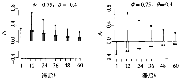They're all typical, and they fit the model we've been talking about.

We'll take the model we're introducing right now. $$ARMA(p,q)\times(P,Q)$$ What does it mean?

• Non-seasonal portion$ARMA(p,q)$
• The season itself.$ARMA(P,Q)$

ARIMA model for unstable seasons

The difference, or the non-stable core step.$s$♪ The season differentials $$\nabla_{s}Y_{t}=Y_{t}-Y_{t-s}$$ And then you combine the difference in your own model, and you can multiply the ARAMA model for it has a model.

• Seasonal cycle$s$
• Non-seasonal steps$ARIMA(p,d,q)$
• The order of the season$ARIMA(P,D,Q)$ It's a big model.

Seasonal ARIMA model recognition, preparation, testing, predictions.

The core approach has been described in the "Structure Identification" section of this paper, the "parameter estimation" section, the "Model Diagnostic" section of this paper. Here's a few separate presentations on the seasonal model.

Seasonal ARIMA model recognition

• Study Time Series Chart ACF PACF Determination of Stable and Periodicity
• Consider normal differentials and try to capture stability.
• Consider the seasonal differentials and try to eliminate cyclicality.
• Study whether the sample ACF is free of self-relevant (the difference is to eliminate all self-relevant)

The sequences of the season ARIMA model after a first-order differential and the seasonal differential often lag behind the positions 1, 4, 5 (in the case of monthly data, by 1, 12, 13) to synthesize the ACF PACF time-series judgement, and have not eliminated the smoothness and cyclicality

Seasonal ARIMA model preparation

We're looking for the MLE formula, and the code will help us calculate the results.

Seasonal ARIMA model diagnosis

Or is it a study of the disability?

Seasonal ARIMA model prediction

As expected, the best way to predict the season model is to use the margin to predict. Consider $ARIMA(0,1,1)\times (1,0)Yeah. $Y t-Y{t-1}=\Phi(Y_{t-12}-Y_{t-13})+e_t-\theta e_{t-1}-\Theta e_{t-12}+\theta\Theta e_{t-13}$$ 一步向前预测就有 $$\hat{Y}t(1)=Y_t+\Phi YOther Organiser$$$US$US$ More steps are the same, and we still need to consider the fact that noise items sometimes include projections in the form of disability, sometimes in the form of self-return. The ARIMA model of the seasons has two parts, one of the pre-time trends, the other of the cyclical segments, and they're our ARIMA seasons.

Seasonal virtual variable

Another method of expressing seasonality is to express a fixed seasonal pattern using non-random regression items. It's possible that this pattern can be eliminated by seasonal differences, but it's also relevant to dynamic models andSimilarity of non-random linear trend models, fixed seasonal models should not be treated with seasonal differentials. If we can find a certain trend, and we can smooth it down, then we don't need to use differential treatment.

Non-random seasonal factors are expressed in the return to the mute variable.$s=4$, the fixed level of the four different seasons is expressed using three dumb variables. To determine whether the non-random season model is used, it is possible to prepare dynamic season ARIMA$(1,0,1)(1,0,1)_s$Models, where seasonal factors are found to be negligible, may consider non-random seasonal models. Examples are given below.

Give Sequence Chart 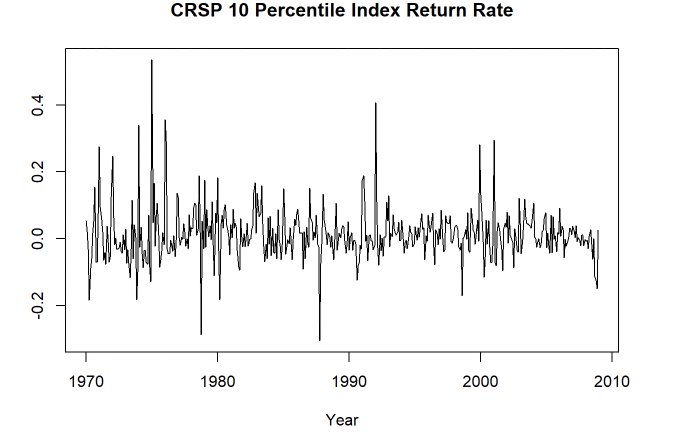Can't see a clear cycle. Make an ACF map. 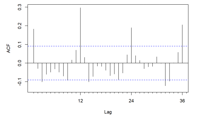The 12th grade lag is clearly not zero, reflecting a cyclical pattern. ARIMA season for dynamic$(1,0,1)(1,0,1)_{12}$ Found sar1 = 0.9882,sma1 = -0.9142 Write as a physical model $$(1+0.0639B)(1-0.9882B^{12})(X_t-0.0117)=(1+0.2508B)(1-0.9142B^{12})\varepsilon_t$$ They can be approximated, which means they can consider a regression model for the seasonal dummy variable, which is essentially a regression problem.Returns to calculate trend The time series features are not considered at this time.

This seems very credible, but in fact, time series data are highly self-relevant, and we'll find this in our analysis of the retrogressive residuals, and it is hasty and irresponsible to take a direct look at trends in the time series and end the analysis.

Retrieval model with time series errors

In statistical analysis, linear regression analysis is one of the most commonly used analytical tools, a linear regression is as follows: $$Y_t=\beta_0+\beta_1X_t+e_t,t=1,2,\ldots,T$$ We're going back to the model and we're going to ask for the disability.$e_t$ Independent as normal distribution

But in the regression analysis of financial implications, time series are frequently present, including the regression analysis we use when going to trends, where they all have non-independent disabilities, based on the disability.$e_t$ The independent and normal distribution of the estimates, like the standard error estimates, the hypothetical tests, are no longer valid. The regression factor estimates are still credible.

Studies have shown that when the disability is positively correlated, the standard error estimate for the regression factor is low, making it corresponding.$t$and$F$Test absolute values for statistics

When?${e_t}$When the ARAMA sequence is flat and reversible, linear regression models can be estimated at the same time as the smooth reversible ARAMA sequence, and standard error estimates, hypothetical tests and projections are available. arima()Function provides xreg= to introduce a regression variable.

If you don't care,${e_t}$The correct estimate of the regression factor for the SE and the correctness of the hypothetical test can be assumed only${e_t}$The structure of the agreement is not considered.${e_t}$Modelling. LikeLinear regression base Section on “Minimum 2x (weighted OLS)”

The basic steps for modelling are:

1. To integrate a linear regression model and test the sequence relevance of the residual
2. If the disability sequence is non-stable in unit, the difference is one-ordered for both the variable and the self-variant. Then we take the first step in the sequence after the difference. If the residue sequence is flat, identify an ARMA model for the residue sequence and modify the linear regression model accordingly.
3. The regression model is estimated jointly with the ARMA model using the maximum semblance estimation method and the model is tested for improvement. The main use is for white noise testing of the disability using Ljung-Box.

Long Memory Model

ACF is an important reference for time series modelling.

• For ARMA sequences, when delayed$k\to\infty$The sample ACF is now zero negative index.
• Theoretically, ACF is not defined for unit root, since the SACF is defined for weak smooth column, and its sample ACF is in sample volume$T\to\infty$Every time$\hat{\rho}_k$Both trend $1.00 (k)> 0)$ 。

There are some flat time series ACFs, though they also lag behind.$k\to\infty$It's zero, but it's slow to zero, only negative.$k^{-\alpha}$ This speed. This represents a slow reduction in the self-relevance of the sequence as it evolves from distance to distance, which is described as a long-term memory time series.

Note that the time series of long memory remains weak and stable, and the unit roots are not called long memory, although they are highly self-relevant from a distance.

In financial time series modelling, long memory models can be considered if the sample ACF values are small but the decline is particularly slow. If the values are large and slow, it could be the unit roots that are not flat, or the ARAMA sequence that has very close to the one.

The typical model of the long memory time series is the fractional balance flat column, the model is the $$1-B ^dX t=\xi t,:-0.5<d<$ 0.5 million of which${\xi_t}$It's zero-average-symmetrical, and white noise.

If we talk about this white noise spreading to the point where we can get it,$ARMA(p,q)$Sequences.$ARFIMA(p,d,q)$ Model called the fractional grade differential ARMA model.

Unstable from mutations

The second reason for non-stableness is that the overall regression function has changed during the sample period. In economics, many of the reasons for this are the sudden changes in an industry as a result of changes in economic policy, changes in economic structure, and innovation. If these changes or “matures” occur, but these factors are not taken into account in the model, they will shake the basis for our predictions and extrapolations.

This section presents the thinking for the two time series regression models to detect mutations.

The first idea is to look for possible mutations from the perspective of the hypothetical test and to pass$F$ The statistics test the significant change in the regression factor.

The second idea is to look for possible mutations from the perspective of prediction: The projection is based on the assumption that the sample was completed by the actual end of the sample period and the results of the projection are evaluated. If the forecast results are significantly reduced in accuracy, a mutation is assumed.

We have just described the unstableness of trends without considering mutations.

What's mutation?

Mutant variations may occur in the general regression function, sudden changes at a given time, or in a long-term evolution.

Unbridled changes in macroeconomic data can result from large-scale changes in macro-policy.

Mutant changes may also result from the evolution of the overall regression function over time, such as slow economic policy reforms and gradual changes in the economic structure.

The methods described in this section for detecting mutations can be used to test sudden mutations as well as mutations caused by long periods of evolution.

The mutation test

One of the methods used to detect mutations is to test the discrete or mutation of the regression coefficient. The specific test will depend on whether the moment of the mutation point occurs.

Known Time

Test of known time mutations. In some cases, you may suspect that a mutation has occurred at a given point in time.

If the date of the possible mutation is known, the double variable cross-entry model can be used to test the zero scenario, which should be non-maritime. For the sake of simplicity, we will consider the ADL (1,1) model, which includes the interpretation variables, the cut-off, the cut-off, and the other variables.$Y_t$♪ And the first step behind ♪ $X_{\iota}$The first step is lagging. Use$\tau$The event is a very important one for the world.$D_\iota(\tau)$ is a binary variable with a value of 0 before the mutation period and 1 after the mutation period, i.e., when$t\leqslant\tau$The blog is also available.$D_t(\tau)=0$, when $t>\tau$时， $D (\tau)=$1.00. The regression equations with binary mutation indicator variables and all cross-cutting items are: $$Y_t=\beta_0+\beta_1Y_{t-1}+\delta_1X_{t-1}+\gamma_0D_t(\tau)+\gamma_1\begin{bmatrix}D_t(\tau)\times Y_{t-1}\end{bmatrix}+\gamma_2\begin{bmatrix}D_t(\tau)\times X_{t-1}\end{bmatrix}+u_t$$ If no mutation occurs during the sample period, the overall regression function should be the same in both stages, i.e. all of which are contained$D_t(\tau)$, and the coefficient for each item should be zero. That is, the zero assumption should be no mutation during the sample period, i.e.$\gamma_0=\gamma_1=$ $\gamma_2=0$I'm sorry. The alternative scenario is that mutations exist during the sample period, which means that the overall regression function is at the mutation point$\tau$Different, i.e.$\gamma_0$、$\gamma_1$、$\gamma_2$At least one is not zero. So, if there was a mutation in the sample period, it could be...$F$Statistical testing

Unknown time

If we don't know the specific time point at which the mutation occurs, then we can consider multiple mutations of known time, and fortunately, the form of integration has been studied.

This improved Zou is usually called Quant Likelihood Ratio (QLR) Statistic (which we will use to indicate this test below), or sup-Wald statistics.

Hypothetical test for external prediction

The test of the accuracy of the model's prediction ultimately depends on its ability to predict outside the sample, i.e., its ability to predict in the “actual projection range” after the model's estimation has been completed.

Hypothetical external predictions (Psueudo Out-of-sample Forecasting) are a method used to simulate prediction models for predicting performance in actual projection ranges. Its approach is simple: select a point of time at the end of the sample range, use data from before that point of time to estimate the model and then use the estimated model to project the observations at the end of the sample. Repeating the above steps at multiple points of time at the end of the sample can provide multiple false predictions and multiple false prediction errors. These errors are used to test whether we are satisfied with the stability of the predicted relationship.

It's also a way to help us judge whether mutation is not a source of stability.

Handle mutations

The handling of mutations is a very complex issue, and we don't have any information here about how to deal with mutations.