Experimental Design Methods: ANOVA, one-factor experiments, and multi-factor experiments

Summary of test design

General

Data for differential analysis; data obtained through a certain design experiment, not some randomly measured data

Pilot design and analysis as a branch of mathematical statistics to study how to design experiments and analyse data;

In essence, the variance analysis examines only one issue: Characteristic values at different levels of different factors We'd like to make some useful judgements by studying this issue.

The purpose of the test design is common.Less experimental workload and lower cost of obtaining sufficient and reliable useful information; his core purpose is to collect data rather than analyse them

Nevertheless, finding a generic test design method that is unshowed can give us some of the better methods of designing a given type of problem, because this type of problem is often very special (in statistical theory).Introduce analysis directly in the test design method

Experiment: Focus on academia Testing: a method to design experiments and analyses

Pilot design is a very applied discipline, and the entire history of experimental design is industry-led.

Development experience

Fisher's variance analysis in farm practice
The Japanese Statistician Taguchi I proposed an experimental design for the production of industrial goods
A balanced design proposed by Professor Wang Yuan, Fang Kai-tae, during China ' s missile development All design methods are designed to reduce the number and cost of experiments in a given situation.

Common terms and models for experimental design

Factors and Levels

In one trial, the variable to be examined is called a factor. Level: Different state of the factor Factors are divided into qualitative and quantitative factors depending on whether the level is continuous or not.

Response

Results from tests The purpose of the pilot design is to study the impact of the interaction of factors and factors on response and the relationship between them The response is sometimes called a characteristic value. A good test is the relationship between getting enough responses and factors at a minimum number of tests.

Random error

It's possible that in the experiment, the amount produced by the experiment has not been included in our study. They're not controlled. Good test designs can significantly reduce random error interference and help us find patterns.

Common statistical models

One of the main reasons for the efficiency of the methods designed by the statistical experiment is that they're very, very efficient. Optimal methods under defined mathematical models; The models used for experimental design are:

Difference Analysis Model
Linear regression analysis model
Non-parameter regression model
Steady regression model We'll talk about it later.

Difference Analysis

We're here.Linear regression baseHe's a regression analysis of an indicative variable, often looking at the effects of the existence or non-existence of a factor.

♪ Though it's ♪Linear regression baseWe see it as a narrow issue of regression analysis, but our chapter will use a new approach.

By studying the origin of the overall variation between data in comparable arrays; finding significant influence factors on things, interactions between factors and optimal levels

We need to ensure data independence. We tend to study the following types of problems in differential analysis models.

Visibility test for mean differences
Effect of the separation of relevant factors on total variability
Interaction between analytical factors
Spacing test

The idea of differential analysis

Here's the data from a trial.

1	2	3	4	5	Mean
89	62	93	71	85	71.4
75	78	60	61	83	80.0
We want to determine which conditions are better observed; if there are no errors in observations, the results of multiple tests under different conditions are the same, and it is natural to judge.
But in fact, the test results are always influenced by errors, and we can't tell whether the differences that we're showing are caused by conditions or errors.
We can describe the fluctuations in the averages from the results of the same set of tests, that is,
$$\begin{gathered}
S_{E}^{2}=(75-71.4)^{2}+(78-71.4)^{2}+\cdots+(83-71.4)^{2} \
+(89-80.0)^2+(62-80.0)^2+\cdotp\cdotp\cdotp+(85-80.0)^2
\end{gathered}$$
For overall indicator fluctuations, the error in the overall average of all tests can be described.
$$\begin{aligned}S_T^2&=(75-75.7)^2+(78-75.7)^2+\cdots+(85-75.7)^2\&=1294.10.\end{aligned}$$
In the case of indicator fluctuations caused by this change in factor, the average of two different levels can be described as the average of the average for the whole.
$$S_{A}^{2}=5(71.4-75.7)^{2}+5(80.0-75.7)^{2}=184.90$$
It's natural. We can see that.
$$S_{T}^{2}=S_{A}^{2}+S_{E}^{2}$$
We can see it, either.$S_A$Still?$S_E$ They all have to do with the number of tests.
Yeah.$S_E$ It uses 10 data, but the two averages were calculated by the remaining ten conditions, two limitations, and he's free. $10-2=8$
Yeah.$S_A$ It uses two data.$2-1=1$
The overall freedom is both.$0$
If the change in condition has a significant impact on the change in the indicator, then we can get it.$S_A$It'll be very big, relative.$S_E$It'll be small.
$$F_{A}=\frac{S_{A}^{2}/f_{A}}{S_{E}^{2}/f_{E}}$$
When the margin is large enough, it can be assumed that the difference in the significance of our tests is not explained by the error.
As we can see from the reasoning above, we need one side.$F$The test will be ours.
Let's do a little research.

Single-factor equation analysis

Model construction

We'll start with a single factor differential analysis. We gave a model profile. $$y_{ij}=\mu_i+e_{ij}$$ of which$y_{ij}$is the specified value $\mu_i$It's the average of several tests at one level and then random error. Which means we think all variables are the same except for the level of factors to be studied. So studying all levels is research.$\mu_i$Variance We can easily transform the above model into the following. $ \begin{aligned} &y_{ij}=\mu+\alpha_i+e_{ij} \ &e_{ij}\sim N(0,\sigma^2) \ &\sum_{i=1}^an_i\alpha_i=0 \end{aligned}$$ 这个模型也是很好理解的 $y_{ij}$是具体的取值 $\mu$是总体的均值 $\alpha_i$是所有的水平对最后取值的影响最后是随机误差至于后面的等式如下就可以证明 $$\sum_{i=1}^an_i(\mu_i-\mu)=\sum_{i=1}^an_i\mu_i-\sum_{i=1}^an_i\mu=n\mu-n\mu=0$$ 还是和我们在第一章干的事情一样改写为矩阵形式 $$\begin{gathered}\mathbf{y}=X\boldsymbol{\beta}+\boldsymbol{e}\e\sim N(0,\sigma^2I_n)\\boldsymbol{h'== sync, corrected by elderman == It's in the form of a matrix that we've studied in the first chapter.

Common statistics in variance analysis

First, give some statistics that are very common in differential analysis. General average $$\overline{y}=\frac{1}{n_ia}\sum_{i=1}^{a}\sum_{j=1}^{n_i}y_{ij}$$ Defines the total squared as follows: $$SS_{T}=\sum_{i=1}^{\alpha}\sum_{j=1}^{n_{i}}(y_{ij}-\bar{y})^{2}$$ It intuitively describes how the whole data is concentrated and all the tests deviate from the overall average. Reordered. $overline{y}{i}=\frac1n\sum{i=1}^ny_{ij}$$ 则定义组内平方和 $$SS_{E}=\sum{i=1}^{a}\sum_{j=1}^{n_{i}}(y_{ij}-\overline{y}{i.})^2$$ 它直观的描述来某个水平下所有的试验偏离水平均值的情况也就是随机误差的影响再定义组间平方和 $$SS_A=\sum{i=1}^a\sum_{j=1}^{n_i}(\overline{y}{i.}-\overline{y}{})^2=\sum_{i=1}^an_i(\overline{y}{i.}-\overline{y}{})^2$$ 它解释了各个水平的试验偏离整体试验均值的程度我们经过一系列运算可以得到下面的定理 $$SS_T=\sum_{i=1}^a\sum_{j=1}^{n_i}\Big[(y_{ij}-\overline{y}{i.})^2+(\overline{y}{i.}-\overline{y})^2\Big]=SS_E+SS_A$$

Assumptions test

What we want to test is a model factor.$A$Whether there are any significant differences in the average values below each level, i.e. $$H_0:\alpha_1=\alpha_2\overset{}{\operatorname*{=}}\cdots=\alpha_a\overset{}{\operatorname*{=}}0$$ Now we can extrapolate the statistics. You can extrapolate to $$E(SS_A)=(a-1)\sigma^2+\sum_{i=1}^an_i\alpha_i^2$$ Therefore... $$E(\frac{SS_A}{a-1})=\sigma^2+\frac1{(a-1)}\sum_{i=i}^cn_i\alpha_i^2$$ It reflects the effects of each level of effect. When hypothetical$H_0$When it was set up, Which means...$\alpha_1=\alpha_2\overset{}{\operatorname*{=}}\cdots=\alpha_a\overset{}{\operatorname*{=}}0$ Therefore... $\frac{{SS}_A}{a-1}\text{是}\sigma^2\text{的无偏估计}.$ $\frac{{S}{S}_E}{n-a}\text{为}\sigma^2\text{的无偏估计}$ Therefore... $$F=\frac{SS_A/(a-1)}{SS_E/(n-a)}\text{接近于1}$$ When the hypothesis doesn't work, it's very obvious that the balance of the group is squared.$SS_A$It'll increase.$SS_E$It reduces the value of testing statistics. So all we need to do is be one side.$F$Test It's in there.$a-1,n-a$It's the expression of freedom.

Estimates

When we reject the assumption that the levels of the factor are different, we need to estimate the size of the difference.$\mu_{i}-\mu_{j}$I mean, I'm going to do an inter-sectional estimation and, of course, integrate the data into the regression analysis. It's easy to know. $ \begin{aligned}\overline{y}{i.}&\sim N(\mu_i,\frac{\sigma^2}{n_i})\\overline{y}{i.}-\overline{y}{j.}&\sim N(\mu_i-\mu_j,(\frac{1}{n_i}+\frac{1}{n_j})\sigma^2)\end{aligned}$$ 因此可以导出 $$\begin{aligned}U&=\frac{\overline{y}{i.}-\overline{y}{j.}-(\mu{i}-\mu_{j})}{\sigma\sqrt{\frac1{n_{i}}+\frac1{n_{j}}}-N(0,1)}\SS_{E}/\sigma^{2}&=\sum_{i=1}^{a}\sum_{j=1}^{n_{i}}(\overline{y}{i.}-\overline{y})^{2}\left/\sigma^{2}-\chi{n-a}^{2}\right.\end{aligned}$$ 最后导出$t$枢轴量 $$\frac{\overline{\boldsymbol{y}}{i,}-\overline{\boldsymbol{y}}{j,}-(\mu_{i}-\mu_{j})}{\sqrt{\frac{\boldsymbol{S}\boldsymbol{S}{E}}{n-a}}\sqrt{\frac1{n+\frac1{n j} $ We won't give up the last compartment. In fact, it's an estimate of the average value difference in mathematical statistics. Don't forget, we have to run a hypothetical test before we talk about estimates of the average margin. If this confidence zone contains zero, it means the average difference is not significant.

Multiple comparisons

The significant differences that we've demonstrated before only show that the levels of this factor have an impact on the indicators, but they don't help us select the most appropriate tests, multiple comparisons and multiple comparisons.$S$The test will help us. First you have to give the factor down the inverted triangle. 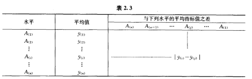The specific sequence software will give us a calculation. Calculate $$D_{ij}(\alpha)=\sqrt{\left(\frac{1}{n_{i}}+\frac{1}{n_{j}}\right)\frac{S^{2}}{n-r}(r-1)F_{s}(r-1,n-r)}$$ If the average of the horizontal indicator is greater$D_{ij}$ Proof of significant differences between the two levels And then we'll fill in the table.

Analysis and interaction of factors

Model description

Control of variables is a difficult thing, and that's why we're going to study the differential analysis of both factors. It's very easy to give the core model of this section. $$y_{ij}=\mu+\alpha_{i}+\beta_{j}+e_{ij}$$ The number of tests at each level of each factor is still to be determined, and if we want to include it, we inevitably introduce the existence of interactions (which are often rarely taken into account in regression analysis, which is already being addressed by the Cyclops). $$y_{ijk}=\mu+\alpha_{i}+\beta_{j}+\gamma_{ij}+e_{ijk}$$

Impact of interactions

We will be followed by a presentation of two factors that do not take into account the interaction and do not repeat the test differential analysis; If we find out

Neither effect is significant.
That's not obvious. It's too big a difference squared.$SS_E$That's because of the error.
We have more confidence in the error control of the experiment. It's very likely that there's a new effect in there that has an impact on the test, and it's often an interaction.

Both factors do not repeat test variance analysis

Or do you have the following definition with the idea of creating squares? Total Square $$SS_{T}=\sum_{i=1}^{a}\sum_{j=1}^{n_{i}}(y_{ij}-\overline{y})^{2}$$ Group squared $US$US$US$US$US$US$US$US$US$US$US$US$US$US$US$US$US$US$US$US$US$US$US$US$US$US$US$US$US$US$US$US$US$US$$US$US$US$US$US$US$US$US$US$US$US$US$US$US$US$US$US$US$US$$US$US$US$US$$US$$$$$US$$$$$$$$$$US$$$$$US$$$$$US$$$$$$$$US$$US$$$$$$$$US$$$$$$$$$$$$$$$$...$$$$$$$$$$US$$$$...$$$$$...$$$$$${i.}-\overline{y}{.j}+\overline{y})^{2}$$ 因素A组间平方和 $$SS_{A}=b\sum_{i=1}^{a}(\overline{y}{i.}-\overline{y})^{2}$$ 因素B组间平方和 $${{SS{B}=a\sum_{j=1}^{a}(\overline{y}_{.j}-\overline{y})^{2}}}$$

New statistics

An assumption that the levels of both factors have a significant impact on the indicator is examined below $$H_1:\alpha_1=\alpha_2=\cdots=\alpha_a{=}0$$ $$H_{2}:\beta_{1}=\beta_{2}=\cdots=\beta_{b}=0$$

Assumptions test

It's easy to give a test count. $$F=\frac{SS_A/(a-1)}{SS_E/(a-1)(b-1)}\sim F_{a-1,(a-1)(b-1)}$$ These coefficients are still limited by freedom. If you want to calculate another factor,$B$The influence only needs the molecule.$A$Replace$B$ Synchronize Freedom Or is it a one-sided test?$F$When you're too big, you reject the assumption.

Estimates

The idea is exactly the same, or do you study the spatial estimates of the average difference? $ \frac/2003/overline{y}{i.}-\overline{y}{t.} (\alpha i-\alpha t)\sqrt {SS E}(a-1)(b-1)}}sqrt}\simt {(a-1)(b-1)}$$ It's very easy to export. If this confidence zone contains zero, it means the average difference is not significant.

Two factors and so forth, repeat test variance analysis.

The model is presented below. $$y_{ij\mathrm{k}}=\mu+\alpha_{i}+\beta_{j}+\gamma_{ij}+\varepsilon_{ijk}$$ Please note that in models where there are interactions, it makes no sense to look at one level of good or bad of one factor, because its good or bad is related to the value of another factor, so we're just...All we have to do is test the existence of the interaction. If there's no way to follow the previous part, if there is, then there's no point in the previous part of the non-interactive study.

We need to test the hypothesis as if $$H_3:\gamma_{ij}=0,i=1,...,a;j=1,...,b$$ Give new statistics $US$US$US$US$US$US$US$US$US$US$US$US$US$US$US$$US$US$US$US$US$US$US$US$US$US$US$US$US$US$US$US$US$US$US$US$US$US$US$US$US$US$US$US$US$US$US$US$US$US$US$US$US$US$US$US$US$US$US$$US$US$$US$$US$$$US$$$US$$US$$$$$US$$US$$US$$US$US$US${A\times B}=c\sum{i=1}^a\sum_{j=1}^b(\overline{y}+\overline{y}{ij.}-\overline{y}{i..}-\overline{y}{..j.})^2$$ $$SS_E=\sum{i=1}^a\sum_{j=1}^b\sum_{k\operatorname{=}1}^c(y_{ijk}-\overline{y}{ij\operatorname{.}})^2$$ 给出$F$检验统计量有 $$F== sync, corrected by elderman == @elder man Or do you use a one-sided test to see intuitively the direction of the test is consistent with the previous section? Now all the work software on differential analysis is available, and no manual calculations are required. At the end of the variance analysis:

The variance analysis is a comprehensive test method, which, as the number of factors increases with their level, the number of combinations increases dramatically and it is not possible to conduct all tests, and we must introduce some of the tests. ^35bacd

Turning over test design.

See the “relevant paragraphs” section of this paper. One of the tests is a more efficient design method.

Arrange tests with a positive tab

A standard due form is shown below $$L_{k}(m^n)$$ of which $k$Other Organiser $m$Indicate the level of the factor $n$Number of indicators Of course, you can use a similar line of thought to indicate a mixed horizontal submission. $$L_{k}(m^{n}\times p^q)$$ Characteristics of the positive submission (reflecting the idea of its balanced experiment)

Write a large matrix, and each row is the horizontal selection of a factor for each test.
Numbers appear as many times as in each column
Each column is balanced by the number, which is the same number of times it appears.

When we're experiencing multiple-factor trials, but we can't do enough, it's often done according to a positive tab, which is created by software.

Direct test design without interaction

Here's how we're going to analyze the calculations based on test data from the positive test. An ordinary test data log is as follows: 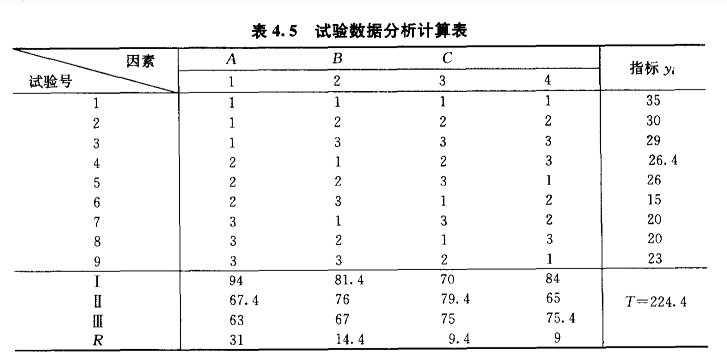The fourth column does not have letters because we only have three factors, but we have a table of four. The blank column reflects the impact of random error, and if the blank column is too different, it must mean that we're missing important influences.

The rightmostbar is the test result, of which$T$It's the sum roman numeral number.$I$ Meaning the sum of the indicator values selected for 1 at all levels in the column where the factor is present (reflecting the average of the values in a group and/or group) $R$That's the factor.IIExtremely bad third-value

In simple data processing, we rely directly on $I.IIThe value of the $3.0 to determine the level of our final choice, and the extreme difference reflects the magnitude of this factor.

And, of course, if you find that some of these factors are not significant, you can make the right adjustments, and you can do the best you can at a smaller cost.

It's obvious that this analysis is too crude, and the conclusions that have been drawn must be retested and never directly accepted.

Direct test design considering interaction

If we want to analyse the interaction in the direct test, the experimental design and treatment programme will change slightly; As a matter of custom, we have the following principles for dealing with interaction.

Ignore advanced interactions
Selectively explore a level of interaction. Usually only those whose effects are more visible, or which the test requires (which interactions depend on experience, difficult to handle)
Use 2-factor experiment to the extent feasible

The usual positive forms are followed by a two-column interactive list used to analyse whether the interaction exists, as shown below. 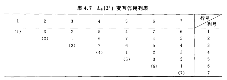All figures in the table are column numbers in the positive table:

If you want to see the interactive column of column 12 from$(1)$ Looking right across from$(2)$ So they look up, and that's how they interact with column three.

It can be seen that if we were to analyse the interaction, many of the columns in the original periodic test could not rank factors, but rather examine the interaction column as a single factor.

At this point in time, the analysis of the existence and size of the interaction would require a study of the obvious impact of the interactive role column on the indicator.

If you look at the interaction, you have to choose a bigger, positive form. $n$Interactive need for factors$n-1$The column interactive column needs to expand the selected positive log to ensure that no multiplicity occurs.

The analysis of the positive results with interactive effects shows the following changes: The original analysis required only an analysis of the impact of the very poor judgmental factors in the various factors, and the extreme difference in the interactive column now reflected the magnitude of the impact of the interaction; the analysis of the other factors did not change;

For the final selection of the appropriate test level:

Not interactive: or the same method of selection as above
The impact of interaction is small: as no interaction
Interactive factors: The selection of its level cannot be considered separately, requiring the drawing of a binary table and a binary chart to be compared before selecting the priority level for the indicator

Multiple indicator test

Many of the tests have multiple indicators to measure the results, and there's a simple approach.

Comprehensive balance approach

The idea is, we're using it as a single indicator, each of which is being analysed separately. Finally, we'll sort out the factors for each indicator. This last step requires subjective observation and trade-offs.

Comprehensive score method

Just as we are.Statistical policymaking The same approach is taken in the “multi-target decision-making” section; some empowerment approach is used to group multiple goals into one, and to carry out related analysis

An analysis of the differences in the design of the test

Here we're going to look at the differential analysis of the positive table test; naturally, it's because the method of subjective selection of the results of the test lacks a measure of certainty about uncertainty. The whole calculation is very simple, or the question of the squared difference.

It's the same rule that gives a high percentage of the statistics to be used this time. Total Square $$SS_T=\sum_{i=1}^n(y_i-\bar{y})^2$$

Square sum of a factor (column change squared) $$SS_{A}=\frac{a}{n}\sum_{j=1}^{a}(K_{j}^{A})^{2}-\frac{1}{n}(\sum_{j=1}^{n}y_{i})^{2}$$ Of which$K_j^A$ Representation factor$A$No. No.$j$the sum of all test values at each level The data in the previous table can be shown as

$$ S_i^2=\frac{\mathrm{I_i}^2+\Pi_i^2+\Pi_i^2+\cdots}{\text{水平重复数}} - \frac { T ^ 2 }{\textbf{数据总个数}}. $$

Sum of error squared $$SS_E{=}SS_T{-}(SS_1+SS_2+\cdots+SS_m)$$

About freedom. $f_T=n-1$ of which$n$It's the total number of tests. $f_i=a-1$ of which$a$is the level of the factor $f_E=n-m(a-1)-1$ It's the level of freedom, the level of freedom, the degree of freedom, the degree of freedom, the degree of freedom. Interactive interactive column as well as thought analysis above

Then we introduce the concept of parity. Medium$MS$value is the sum of squares$SS$ The penalty is freedom. $f$ Which means... $$MS=\frac{SS}{f}$$ So the difference analysis for the test can be calculated.$F$Test statistics for analysis.

Research factors$A$ then $F A}\frac{MS}{A}}{{MS}That's right. Other factors are the same. That's how we do the differential analysis of the positive test.

Difference analysis, all empty columns and the effect of error items

Factors that have a disproportionate impact include errors

A positive table without an empty column is not capable of a variance analysis and requires a repetition of the error in the time estimate.

Repeated tests and repeat sampling

There are no empty columns in the active table and it is not possible to use it to calculate the error of the test. In the event of a decision not to use a larger positive submission (the selection of a large positive submission would result in a sharp increase in the number of tests), the error of the repeated test may be used as a test error. Of course, if there's any other reason to repeat the experiment, that's how it works.

The place where the data are being filled in the test form will change in the case of repeated tests or repeated sampling as follows: 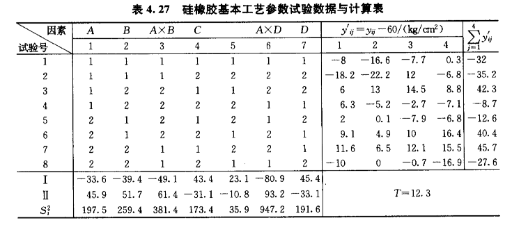The calculation of our data on the table is basically unchanged. These calculations usually let the software go.

Flexible use of positive returns

Mix positive tabs with parallels

It's a common method used to construct positive tabs at different levels. $$L_{k}(m^{n}\times p^q)$$ This part of the job is no longer manual. Give us the number of factors we need, the level of each factor, and the statistical software will give us the positive forms we need, and we don't need to know.

The only thing we need to notice here is:When the level of the factor is identical, the primary relationship of the factor is determined entirely by the size of the extreme R. When levels are not exactly the same, direct comparisons are not possible because when quantitative factors have the same impact on indicators, the factors for multiple levels should be much higher. So we need to use the coefficient to convert the extreme.

Proposed horizontal approach

To add some less horizontal factors to some more virtual ones so that the less horizontal ones can be ranked in the positive tables that we need. Medium It's very simple. Let a certain level of the factor repeat as a new level. Medium

Additional notes:

Given the different levels of factor D and other factors, it would be inappropriate to use the extremely poor R to compare the order of the factor (conversion factor). However, the use of differential analysis can still yield reliable results.
While the horizontal approach has expanded the use of the positive instrument, it is worth noting that it is no longer a positive table after the proposed horizontal changes, and it loses the nature of the balanced mix between the levels of the various factors

Delineation of factors

The method of putting higher-level factors into lower-level positive tables.

Immediate Law

We're going to experience too many different levels of testing in large-scale industrial experiments, too many tests on a positive table, and we need to do it in stages. There are common ideas.

Reduction factor: fix certain factors not tested in the first table and change the level of this factor in the second table
Reduced level: part of the level of a factor does not test in the first and in the second allows the best in the first to be compared with the remaining untested level
Combination factor: to combine multiple factors, if they are not significant, then there is no direct need to continue the split test. It'll take us to do it in parallel to get the final results.

Flow method

A differential analysis method focused on the interaction of some and others For example, in chemical tests there are formulation factors (raw materials, matching, etc.) and process factors (processing time, temperature, etc.) there must be two types of interaction; but their internal interactions can often be ignored. In the experimental design, we consider only interaction between classes, not interaction between factors within classes. Finally give the margin analysis table.

The core of the two categories of differential analysis is the proper use of statistical software, and all we need to do is look at the final methodological analysis table and reschedule the tests as appropriate.

even design

evenly designed presentation

We first presented the variance analysis of the full-scale test, and then the problem of the contemporary design due to the high level and number of elements, which was also presented to address the inadequacy of the original experimental design methodology.

The characteristics of the current table tell us that the number of active tests is double the number of squares of horizontal numbers, which means that the increase in our level is related to a flat increase in the number of tests, which, if the level is too high, will soon reach an amount that we cannot afford.

However.Multiple-level experiments are also frequent, and we need new experimental methods, which raises the issue of even design. The flat design is Fong Kai-tae, and Prof. Wang Yuan took up the idea of digital theory in his research on missile design tests. It is an application of the pseudo-Montecaro method (formerly Monte Carlo is a random generator, and the pseudo-Monte Carlo idea is that it is supposed to produce a hyper-equilibrium sequence).

The original experimental design idea.

evenly dispersed: the test sites are distributed evenly within the test range, allowing for adequate representation of each test point
Accompanying: makes it easier to analyse the results of the tests, to estimate the impact of the factors on the indicators and to identify the main contradictions affecting the change of things The pilot design is already the best solution for meeting these two test conditions, but if we ignore the requirement of alignment and comparability, even design is proposed.

even design sheet

The flat sheet is the $${\operatorname*{U_7}}(7^6)$$ Of these, the first corner mark 7 means the number of tests, the number in brackets 7 means the allowed level, the upper mark 6 means the permitted number of factors, the U means the uniform design, and the symbol in the table means that only the L is replaced by the U.

Using a uniform design, each level of the factor is tested only once, and when the level increases, the number of tests increases with the level. The number of tests has changed from squared to linear.

Each flat design table is accompanied by a table of usage, calculated by the predecessor on the basis of some rule, which shows how we select the appropriate columns from the design table and the degree of homogeneity of the test programmes made up of these columns. Give${\operatorname*{U_6}}(6^6)$ And the corresponding usage forms are:

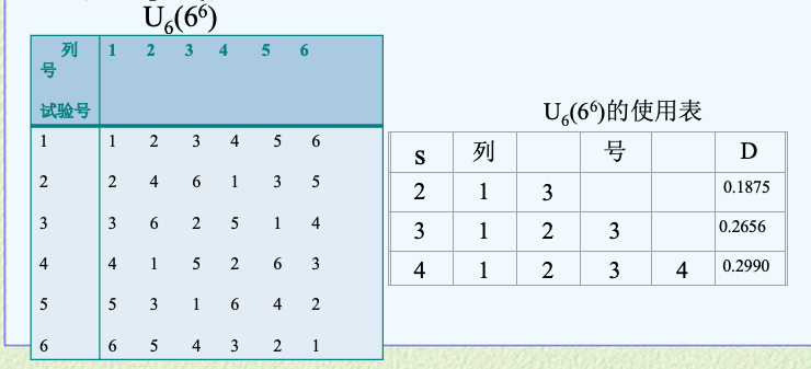
There is no difference between the test table on the left and the interpretation of the active test design table on the right, and the use table on the right tells us that 13 columns and three factors and 123 columns should be used for both factors.

Draw odd tables into the last line and get even tables less than it, and use the table unchanged

In particular: In chemical experiments, low-level and low-level encounters may be unreactive, high-level and high-level encounters may be over-reacting, and we need to adjust the numbering of the level; based on the principle of uniform design tables, he cannot simply change the order of the level to the same level as the original test design table, but only smooth it in the order of a circle, which requires our attention.

Analysis of the results of the flat design test

Since the flat design no longer takes into account the full comparability of the present test,The test results are processed using regression analysis.• Linear regression or multiple regression analysis.That's using the interpretation model in the regression analysis to achieve the outcome analysis.

A regression test may be conducted in the regression analysis to determine the significance of the factor in the model, depending on the size of the regression square;

Where there is no correlation between the factors, the fact that the factor is back to square size also reflects its importance for the impact of the test indicator. It's usually done with computers.

All techniques of regression analysis can be used for uniform design tests, but it is important not to use the results of differential analysis techniques to analyse even design, with too many features and too few observations leading to no results.