Common Statistical Tests Are Linear Models

This post is a good article from Jonas Kristoffer Lindeløv. Common statistical tests are linear models The original text reveals in a very shallow way an amazing simple truth in statistics: most commonly used statistical tests (t-test, related analysis, ANOVA, calculator tests, etc.) are exceptions to linear models.

The questions in this article can also be addressedLinear regression base: linear model, minimum 2x2 estimate and regression diagnosis、Linear regression step: proposed alignment, model selection and co-line SexHow the concept of a relatively close read together is developed in different contexts.

Common statistical tests are linear models

Core concept: Linearness of everything

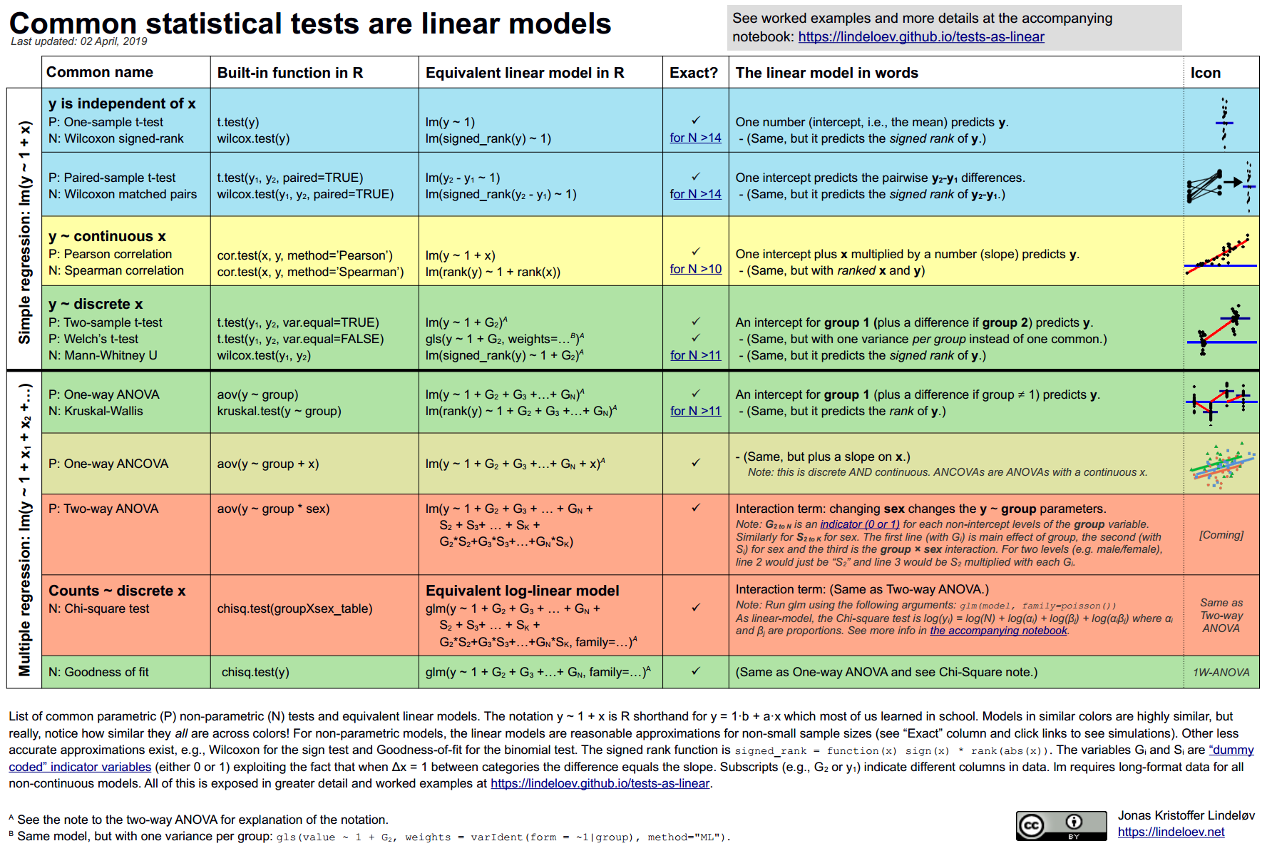
Most commonly used statistical models (t-test, coordination, ANOVA; chi-square, etc.) are either linear models or similar ones. We do not have to remember the assumptions and formulas of each test in the back, because they can be attributed to the formulas that were taught in high school:

$$y = a \cdot x + b$$

This simple aesthetic sense lowers the threshold for understanding statistics. The linear models at the bottom are consistent, whether they are frequency, Bayesian or on the basis of replacement.

For what is called the "non-parametric tests", we can also understand in a more intuitive way: They're usually just...Zirconium (rank-transformed) The corresponding parameter tests run on the data. Instead of considering the non-parametric test “no assumptions are required”, it is understood as “calculating in rankings (ranks)”.

This view is summarized in the figure below (click on page). Look.PDF Version）：

Relevance (Pearson and Spearman)

Theory: as a linear model

The essence of the relevance analysis is to find the best possible line. The model formula is as follows:

$$y = \beta_0 + \beta_1 x \qquad \mathcal{H}_0: \beta_1 = 0$$

That's what we know. $y = ax + b$I'm sorry. In R languages, we usually write y ~ 1 + xThat means... $y = 1 \cdot \beta_0 + x \cdot \beta_1$I'm sorry. It's got to be cut by the cut, no matter what.$\beta_0$) and tilt ( )$\beta_1$(c) Composition.

Rank-Transformation and Spearman

Spearman, the coefficient is actually right. $x$ and $y$ Conduct& Change (Rank-Transformation) Post-Pearson correlation coefficient:

$$rank(y) = \beta_0 + \beta_1 \cdot rank(x) \qquad \mathcal{H}_0: \beta_1 = 0$$

The term "Rank" is used to replace the value with their size ranking (minimum 1 and second, small 2...). Although Spearman's p value was only approximate at the time of the small sample, when N > The time is usually sufficiently accurate.

R-Class: Pearson

Run the R code below, you find a linear model (lm) $t$, $p$ Value & & & & Inline cor.test Exactly.

The difference is:lm It gives a slope, and... cor.test The relevant coefficient is given. $r$I'm sorry. If we standardize the data (SD=1), the slope is equal to $r$。

# Built-in t-test
a = cor.test(y, x, method = "pearson")

Equivalent linear model: y = Beta01 + Beta1x
b = lm(y ~ 1 + x)
On scaled vars to recover rc = lm(scale(y) ~ 1 + scale(x))

R Code Contrast: Spearman

The same logic applies to Spearman's connection, just to do the data first. rank() Change:

# Spearman correlation
a = cor.test(y, x, method = "spearman")

Equivalent linear modelb = lm(rank(y) ~ 1 + rank(x))

Average (One Mean)

Theory: as a linear model

Single sample T test (One-sample t-test) tested whether the average sample value is significantly different from 0. It's actually a...Only the cut.Linear model:

$$y = \beta_0 \qquad \mathcal{H}_0: \beta_0 = 0$$

Not here. $x$Or... $x=0$♪ So the rest ♪ $\beta_0$ It's the average.

For non-parameters Wilcoxon Symbolic Test (Wilcoxon signed-rank test)It's the same principle. It's just applied.Symbolic (signed ranks) Data:

$$signed_rank(y) = \beta_0$$

R Code Contrast: Single Sample T Test

# Built-in t-test
a = t.test(y)

Equivalent linear model: intercept-onlyb = lm(y ~ 1)

You'll find out. lm(y ~ 1) , the estimated value of the amplitude item (Estimate) is the mean, the t and p values are also equal to t.test The results are perfectly consistent.

R Code Contrast: Wilcoxon Symbol Check

# Built-in
a = wilcox.test(y)

Equivalent linear model
b = lm(signed_rank(y) ~ 1)
Bonus: also works for one-sample t-test on signed ranksc = t.test(signed_rank(y))

Use lm Not only do you get a p-value matching, but you get a "mean sign" directly, which is a more intuitive number than a simple W statistical figure.

Other common testing summary

In addition to the two examples mentioned above, other common statistical tests can be mapped into linear models. To keep the paper simple, a summary cross-reference is provided below, with a link to the original text for detailed extrapolations and codes.

Statistical Test (Test)	Linear Model Formula (Simpleted LM)	Original Link
Double means (Independent t-test)	$y = \beta_0 + \beta_1 x$ ($x$ (is a subcategory variable)	Link
Three or more means (One-way ANOVA)	$y = \beta_0 + \beta_1 x_1 + \beta_2 x_2 + ...$ (Perfect variable coded)	Link
Analysis of the differences (ANCOVA)	$y = \beta_0 + \beta_1 x_{categorical} + \beta_2 x_{continuous}$	Link
Scale to calorie (Portions / Chi-square)	$\ln(y) = \beta_0$ (Log-linear Models, returns using Poisson)	Link

Summary

Understanding the linear model relationships behind these tests allows us to reduce our reliance on specific "test names" and to focus on model construction. Whether t or complex ANOVA, they answer the same question: Are my model parameters significantly not zero?

Thank you. Jonas Kristoffer Lindeløv Provides a brilliant perspective.

Original Link: Common statistical tests are linear models
Python Version: Tests as linear (Python)
GitHub Repository: lindeloev/tests-as-linear