Interpretable Machine Learning: Model Explanations, SHAP, and Counterfactual Methods

This English version was machine-translated from the Chinese original. Technical terms may require verification.

Between the beginning.

Introduction

Machine learning has great potential for improving products, processes and research. But computers are often unable to explain their predictions, which is an obstacle to learning by machine. And that's what we're trying to solve here.

We'll deal with the basic presentation, then we'll discuss interpretative models, generic methods, and finally a sample-based interpretation.

Our focus is on the mechanical learning model of table format data (also known as relational or structured data), which basically does not address computer visual and natural language processing tasks. It's only about monitoring learning.

This is not about the latest studies that explain machine learning, but about the more mature methods.

Finally, we would like to stress one point: Multimodel integration has now become a necessary weapon for major machine learning competitions, and most of the winning models are model integration or very complex models, such as upgrading trees or deep neural networks, which actually reduces the model ' s interpretability significantly.

Terminology

In order to avoid ambiguity, some agreed terms are given here.

• Algorithm It's a set of rules that machines follow to achieve a specific goal.
• Machine Learning (Machine Learning) A methodology that allows computers to learn from data to make and improve projections
• Learner (Learner) or Machine Learning Algorinthm is a program used to learn machine learning models from data.
• Machine Learning Model (Machine Learning Model) It is a learning program that maps input to prediction, which can be a linear model or a group of weights of a neural network. Model (Model) can also be called "Prognator" (Predictor), based on a task that can be divided into "Classifier" or "Regression Model"
• Blackbox Model (Black Box Model) It's a system that doesn't reveal its internal mechanisms.White Box (white Box)In this book, it's called an interpretable model. The model's unconnected interpretation treats machine learning models as black boxes.
• Interpretable Machine Learning Means the methods and models that enable the machine to learn the behaviour and predictions of humans.
• Dataset (Dataset) It's a table containing data from which the machine has to learn.
• Example Show as a line in the data set
• Characteristics (Features) is used to predict or classify inputs. Characteristics as columns in data sets
• Target (Target) It's the machine that has to learn to predict.
• Machine Learning Job (Machine Learning Task) A combination of data sets with characteristics and targets
• Forecast It's a machine learning model based on a given feature.

Dataset

Here we present the data sets that will emerge from the following examples. There are no examples to explain how machine learning is hard to understand. There are many examples that will help us understand how.

We will use different data sets for different tasks: classification, regression and text classification.

Data files already have project folders with original books on Github Medium

Bicycling (return)

This data set is derived from the UCI Machine Learning Database, which is publicly provided by Capital-Bikeshare with daily counting of bicycle rentals, Fanee-T and Gama adding weather data and seasonal information

We don't use all the data set features, but the features we use are basically covered.

• Number of bicycle rentals
• Various dates, such as seasons, holidays, calendar days, working days
• Various weather markers, such as temperature, humidity, weather (close rain and snow), wind speed

YouTube garbage review (text classification)

For example, we use 1956 comments from five different YouTube videos, using YouTube API

These comments are manually marked as garbage comments or regular comments. The trash comment is code "1" and the normal comment is code "0".

Risk factors for cervical cancer (classification)

The cervical cancer data set contains indicators and risk factors for predicting whether women will suffer from cervical cancer. These characteristics include human and statistical data (e.g. age), lifestyle and medical history.

Our main features are:

• Basic demographic data: age, age of first sexual intercourse, number of sexual partners, number of pregnancies
• Drugs and drug data: smoking, smoking age, hormonal contraception, hormonal contraception, IUD, IUD
• Disease data: Sexually Transmitted Diseases (STDs), Number of STDs diagnosed, time since first STD diagnosis, time since last STD diagnosis
• Target output: The results of the biopsy are “health” or “cancer”.

Explanatory

Explanatory definitions

There's never been a mathematical definition of interpretativeity. We've given some thought here.

Miller's informal definition of interpretativeity is the extent to which one can understand the reasons for decision-making.

Another explanation is: interpretability means the degree to which people can predict the results of models in a consistent manner.

The higher the interpretability of machine learning models, the easier it is to understand why certain decisions or predictions are made. If decision-making on one model is easier to understand than on another model, it is more explanatory than on another model.

Interpretability can be described in terms of both Interpretable and Explicable terms, but they are distinguished. We will use Expressable to describe the interpretation of individual case predictions. Interpretable is the interpretation of the whole model.

Importance of interpretability

When it comes to forecasting models, we need to weigh: we just want to know what the projections are. Or do you want to know why you made such a prediction? Both tend to be at both ends of the balance.

People want models to be explained for a few reasons.

• Human curiosity and learning ability We're just curious about the answer to that.
• Machine.Impact of decision-making on people ' s livesThe bigger the machine, the more important it is to interpret its behavior.
• The goal of science isAccess to knowledgeThe model itself should be a source of knowledge. Interpretability makes it possible to extract these additional knowledge captured by models.
• Machine learning models only work when they can be explained.Debugging and auditing

In some cases, we often do not need interpretativeity, but rather a better prediction.

• Explanatory is not required if the model has no significant impact
• We don't need to explain when the problem is being studied in depth.
• Interpretability may make it possible for a person or process to manipulate the system, and people may modify their own characteristics in the light of the results of the interpretation, most commonly in the context of credit reviews Nuclear

Classification of explanatory methods

Methodologies for machine learning interpretability can be classified according to various criteria.

Introsic or later?

Essential interpretability refers to machine learning models, such as short decision tree or thin linear models, which are considered to be interpretable because of their simple structure;

Ex post interpretative means the application of an interpretative method after model training, e.g. the importance of a replacement feature is an ex post interpretative method.

The after-action approach could also be applied to models that are essentially interpretable. The sequence behind us is from the essence of the interpretation model to the ex post interpretation problem.

Essential interpretability is usually specific to certain categories of models (Model-specific), and ex post interpretation methods are often irrelevant to models (Model-agnostic).

Local or global?

Does the method of interpretation explain individual case predictions or whole model behaviour? Or is it in between?

Explanatory scope

Algorithm Transparency

Algorithmic training produces predictive models, and each step can be evaluated on the basis of transparency or interpretability

Algorithmic transparency refers to how algorithms learn models from data and what relationships they can learn. Transparency in algorithms requires knowledge of algorithms rather than data or learning models. He's related to interpretability, but he's two concepts.

Global, corporate model interpretability

Once you understand the whole model, you can describe it as an interpretable one.

The interpretability of this level is based on an overall understanding of model characteristics and each learning component (e.g. weight, other parameters and structures) how the model is made.

In practice, however, it is difficult to achieve the interpretability of global models, and any model beyond several parameters or weights is unlikely to be suitable for human short-term memory. Normally, when people try to understand a model, they consider only a part of it, such as weights in linear models. This is the section on "Global Model Interpretability at Modular Level."

Global model interpretability at the modular level

While global models are usually not interpretable, there is at least an opportunity to understand some models at the modular level.

Not all models can be explained at the parameter level. For linear models, it is explained that the weights are in part those of split nodes and leaf nodes for trees.

For example, linear models seem to be perfectly explained at the modular level, but the interpretation of individual weights is interrelated with all other weights. The interpretation of individual weights has always been accompanied by a footnote, namely, “Other input characteristics remain of the same value”, which is unrealistic in many practical applications. Still, it's a good model.

The explanation at the modular level is that we are focused on research, because human understanding prevents us from understanding a model with a large number of (three or four) parameters.

Local interpretability of individual projections

When global models cannot be explained, we may wish to look at an example.

Check the model ' s prediction for a particular input and explain the reasons. If you look at individual predictions, then the behavior of this original complex model may be more pleasant.

Local interpretation is more accurate than global interpretation. In the subsequent introduction, the chapter on “Model-independent methods” could make predictions of individual examples easier to interpret.

Partial interpretability of a set of projections

Very naturally, we can now explain individual examples, if we get an example group, using a separate local interpretation method, and then list the results for the whole group or aggregate the results. You can explain the model to a great extent.

Nature of interpretation

We have to explain the predictions of machine learning models. To achieve this, we rely on an interpretation method, an algorithm that generates interpretation.Interpretation usually links the characteristic values of the example to its model prediction in a way that humans understand.

We examine the methods of interpretation and the nature of the interpretation, which is used to assist in determining whether an interpretation is good or not, but there is still a lack of quantitative assessment of whether it is good or not.

Nature of means of interpretation

• Expressive Power: is the “language” or structure of the interpretation that the method can produce
• Translucency: Describe the extent to which the method of interpretation relies on looking at machine learning models (e.g. their parameters). Since the high-transparent method of interpretation and the model, the low-transparent method needs only to modify the input and then observe the prediction
• Portability: Describes the range of machine learning models using the means of interpretation, the larger the nature, the better
• Algorithmic Complexity: describe the computational complexity of the method of generating the interpretation

Nature of individual interpretation

• Accuracy: If an interpretation is to be used to predict, a model of high accuracy is required, which is less accurate if only an explanation is required.
• Solidity: explain the approximation of black box models
• Consistency: How different is the interpretation between models trained on the same mission and producing similar predictions
• Stability: How similar an interpretation can be between similar examples
• Understandability: What is human understanding of interpretation?
• Determination (Certainty): explain whether it reflects certainty in machine learning models
• Importance (Degree of Importance): The extent to which the interpretation reflects the characteristics or partial importance of the interpretation
• novelty (Novelty): explain whether the data examples to be explained are from a "new" area far from the distribution of training data
• Representation (Reprecentativeness): How many instances can an explanation cover

A humane interpretation.

The explanation is obvious, and there's nothing that traditional machine learning can do about it.

As an explanation of events, humans prefer short explanations (only 1 or 2 reasons), which compare the current situation with the non-occurrence of events, especially where unusual causes provide a good explanation.

When you consider the need for an interpretation of all the factors of prognosis or behaviour, you do not need a humane interpretation, but rather a complete attribution of cause and effect.

We're here to introduce what we're doing about people, and we're trying to get a quick understanding of what our models are doing.

• Interpretation is contrasted. Humans do not usually ask why some predictions are made, but why they are made rather than another. So the good explanation is...Emphasizing the greatest differences between interested and target audiences。
• Selective interpretationOne does not want an explanation of the actual and complete causes of the events covered. We are accustomed to choosing one or two of the possible reasons for interpretation.Even though the real situation is complex, only one or three reasons are given.
• The explanation is social. : For a specific group of people, we need different interpretations, different people understand and focus on their audiences
• The point of explanation is abnormality.There is greater interest in explaining the causes of the events, which are very unlikely to occur, but do. Eliminating these unusual causes will significantly change the outcome (anti-fact interpretation). The anomaly is a very good explanation, even if models don't think so, but people think so.
• The explanation is true. : the interpretation should predict events as honestly as possible
• A good explanation is consistent with a priori knowledge of the subject.: Humans tend to ignore information that is inconsistent with their a priori knowledge, an effect known as confirmation deviations (see A/CN.9/WG.III/WP.36, paras. Even if you think your interpretation is true, it's not likely to be accepted if you don't know a priori.
• A good explanation is universal and probable.: Universality can be easily measured by characteristic “support”, i.e. the number of instances to which the interpretation applies divided by the total number of examples. Let's give the most common explanation possible.

Explanatory model

The simplest way to achieve interpretability is to use only a subset of algorithms that create interpretable models. Linear regression, logical regression and decision-making trees are commonly used as interpretable models.

The contents of this chapter will focus on these interpretive models, we will focus only on our interpretation, not on the rationale, and we will simply review and provide a jumpover for those models that have been studied in the basics.

Characteristics of the model: If the link between characteristics and objectives is linear, then the model is linear.

Models with single-modular constraints ensure that the relationship between the characteristics and the target results remains in the same direction throughout the characteristics: either the increase in the feature values will always lead to an increase in the target outcome or will always lead to a decrease in the target result. Modularity is useful for model interpretation as it makes understanding relationships easier.

Some models can automatically contain interactions between features to predict target results. You can create interactive features manually, and you can include them in any type of model. Interaction enhances forecasting performance, but too many or too complex interactions undermine interpretability.

Some models only deal with regression, others only with classifications and others both.

The usual models we're going to introduce are the following.

Algebra	Linear	Monophonic	Interactive	Tasks
Linear regression	Yes	Yes	No	regr
Logical regression	No	Yes	No	class
Decision Tree	No	No	Yes	class,regr
RuleFit	Yes	No	Yes	class,regr
PARK Soo Bayes.	No	Yes	No	class
k-nearest neighbour	No	No	No	class,regr

There is no clear line between the interpretable and the non-explainable models and it needs to be viewed rationally

Linear regression

The acceptance of linear models does not explain our online regression base.

Explanatory characteristics

The interpretation of weights in linear regression models depends on the type of characteristics.

• Numerical characteristics: Adding a unit of numerical features will change the estimated results according to their weight
• Class II characteristics: Each example uses the characteristic of one of two possible values, while the other value is considered a reference category. The reclassification of the feature from the reference category to the other category would change the estimated result according to the weight of the feature.
• There are several categories of classification characteristics: characteristics with possible values in fixed quantities. Usually we need to use one-hot code to handle multi-classification features. Then we'll use the explanation of the characteristics of the second classification.
• Intersection: Intersection is the characteristic weight of the "continent feature" and for all examples is 1 and is explained as the projection for all numerical characteristics of zero and classification of cases under the reference category

Based on the above explanations, we can give some explanation text templates, and use templates to automatically generate model coefficients

Explanation of numerical characteristics：$当所有其他特征保持不变时,特征x_k\text{ 增加一个单位,预测结果 }y\text{ 增加 }\beta_k\text{。}$ Characteristics of the classification：$当所有其他特征保持不变时,将特征x_k\text{ 从参照类别改变为其他类别时,预测结果 }y\text{ 会增加 }\beta_k\text{。}$

In the case of interaction, the question of the interpretability of coefficients is clearly complicated. We introduced a regression model with interactive entries. $$Y_i=\beta_0+\beta_1x_i+\beta_2u_i+\beta_3w_i+\beta_4x_iw_i+\epsilon_i$$ The situation is different.

• Two binary variables interact.
• A binary variable and a continuous variable interact.
• Two consecutive variables interact

Interactivity of two binary variables: first calculation of the expected values for all binary interactions and comparison of these expectations, all regression factors can be explained by the difference between the expected values

Intersection of continuous and binary variables: Depending on the context of the interactive item, different lines of regression can be obtained, and differences of regression lines can explain the significance of the regression factor

(b) The question of the interaction of two consecutive items: if we keep the original two volumes at the same time, any single variation of a variable from one variable will affect the variable by two coefficients;The coefficient of the joint item reflects the sum of the effects of the two variables at the same time as the two variables were converted more than the single variable.

Visually interpret linear regression

Linear regression models have a lot of options for visual interpretation.

Weight Plot

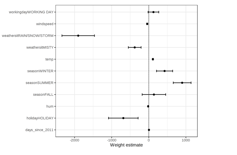
Information on the weight table (weight and variance estimates) can be visualized in the weight chart

In order for them to be comparable on the axis, we need to standardize before using this visualization method.

As shown in the figure below:

Effect Plt

The effect map is another visualization that we do not need to standardize, but multiply the weights of linear regression models with the actual characteristic values; then we draw the Boxplot for each characteristic effect and place it in a comparable axis.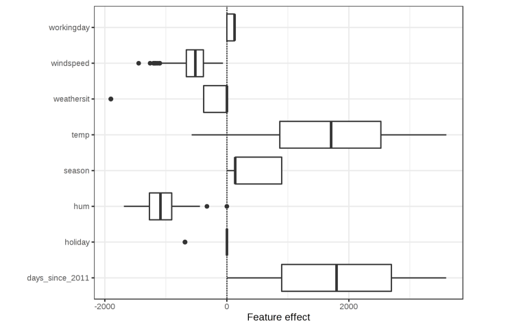

Explanation of individual case projections

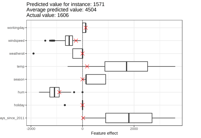
All that has been described is the overall interpretation model, and now we would like to be able to explain the prediction of a single case, why his projection is small (very large) and just to study the characteristic effects.

When we calculate the effects of the characteristics of this example, it is clear who has the most significant effect of combining their criteria in the effect map, and Hum is the main reason for the smallness of this example.

Linear regression discussion

In terms of the nature of what constitutes a "good" interpretation, linear models do not create the best interpretation. They are contrasting, but the reference example is a data point constructed, where all numerical features are zero and the classification feature is set as their reference category, which is usually a manual and meaningless example and is unlikely to appear in your real data or reality.

Linear regression increases prediction modelling to a weight, makes prediction generation transparent and ensures that the best weight can be found, and allows for confidence-building, testing and reliable statistical theory

From the perspective of predictive performance, linear models are usually not so good, and it is not convenient that each non-linear or interactive must be artificial and provided to the model explicitly as an input feature.

The diversity of characteristics in the real world and the absence of those characteristics and interactions will significantly influence the interpretability of models.

Logical regression

Basic knowledge to refer to Logistic returns When we studied the logical regression, we studied its interpretation methods like the Logistic regression coefficient.

Decision Tree

The decision tree is a very good machine learning algorithm that works very well on non-linear questions and the interaction of features. Introduction to Machine Learning and Monitoring Learning: Decision Tree

Explain the decision tree.

Visual decision tree

The decision tree wants to be explained at the very heart of this.

The major software provides visualization of an ordinary decision tree, which is the basis of our understanding of the decision tree's interpretation.

Interpretation

The template to explain the decision tree is: $\text{“如果特征 }x\text{ 比阈值 }c\text{ [小/大] AND ...,那么预测结果就是节点 }y\text{ 中实例的平均值。”}$

Characteristic importance

In the decision tree, the overall importance of a feature can be calculated by passing through all the divisions of the characteristic and measuring how much difference or Gini has been reduced relative to the parent node. The sum of all materiality is scaled to 100, which means that each materiality can be interpreted as part of the importance of the overall model.

Tree decomposition and individual predictions

Individual predictions of the decision tree can be explained by dividing the decision path into the composition of each characteristic. We can interpret projections by tracking decisions through trees and by adding contributions to each decision point.

From the predicted mean of the root node, the projection is modified in each division until the leaf node is reached, and the formula can be expressed as $$\hat{f}(x)=\bar{y}+\sum_{d=1}^D\text{split.contrib}(d,x)=\bar{y}+\sum_{j=1}^p\text{feat.contrib}(j,x)$$ On the basis of the additions and subparagraphs of this formula, it is possible to determine which division has a significant impact, while adding the multiple division of characteristics together, it is possible to determine how much each feature contributes to the projections.

Decision tree discussion

The tree is very structural.Appropriate interaction between features in capture dataI don't know. There's a natural visualization and there's a good interpretability.

Trees can't handle linear relationships.I don't know. Enter any linear relationship between the feature and the result that must be approximated by partitioning to create a step-step function

The trees, the lack of smoothness, are rather unstable, the trees too deep are hard to understand.

RuleFit

The linear regression model doesn't take into account the interaction between the features, so we want to look for something that's...It's like a linear model that's simple and interpretable, but that's where it comes together.This is RuleFit.

RuleFit learns rare linear models with original features and many new features (decision-making rules), which capture the interaction between original features.RuleFit automatically generates these features from the decision tree and can calculate their significance.

The rule of decision-making itself is a sort of classification algorithm, but it's only working.

Method of interpretation

Since RuleFit eventually estimates a linear model, its interpretation is the same as that of the “conventional” linear model. The only difference is that the model has new features derived from decision-making rules. The decision-making rule is a binary feature: a value of 1 indicates that all conditions of the rule are met, otherwise the value is 0.

For linear items in RuleFit, the explanation is the same as in linear regression models:If a unit is added to the feature, the forecast results change with the corresponding characteristic weights.For decision-making characteristics it should be ** if a decision-making rule $r_k$ All conditions are applicable. $\beta_k$ **

RuleFit Discussion

RuleFit Automatically cross-add features to linear modelsI don't know. It therefore addresses the issue of linear models that must be manually added to the interactive function and helps to model non-linear relationships.

He's a very effective method of automatic interaction, but only those decision-making interactive items are identified, but he'll generate too many interactive items, and we'll need to compress them with something like LASSO.

There's a paper that claims that RuleFit is very good -- close to the predictions of random forests, but it's hard to be recognized that if it was really good, he wouldn't be so natural. First Name

The end product of the RubeFit process is a linear model with additional fancy features (decision-making rules). And the linear model explains the need to keep other features unchanged, and there is a real risk of conflict in decision-making rules.

PARK Soo Bayes

PARK Soo Bayes's explanation is based on the distribution of each feature, and we just need to look at the probability.Machine Learning Introduction and Monitoring Learning: The Bayesian Catalogue Very easy to understand.

k-nearest neighbour

We talked about k-near Neighborhood. Introduction to Machine Learning and Monitoring Learning: k - Recent Neighborhood The "sample-based interpretation" section of this paper is the closest possible reference.

Method of interpretation not related to the model

Before you start.

Separating the interpretation from the machine learning model (= non-model-related means of interpretation) has the advantage of being very flexible, and we use any model we like. At the same time, it is easier to compare interpretability between models, as the same methods can be used for any type of model.

The alternative to a model's unconnected means of interpretation is to use only an interpretable model, whose shortcomings are clear and at the expense of predictive performance.

The model of interpretation gives more vision to machine learning, and in the traditional machine learning method, we're looking at how we can learn from it.WorldCollectionData♪ With ♪LearningMethod obtainedModelAnd finally, using models.ProjectionsI don't know. Now we've added a layer of predictions and models that can be made by models themselves.Human understanding.

This multilayered abstract structure allows us to understand the differences in methodology between statisticians and machine-learning specialists.The statisticians handle the data layer, they skip the black box model layer, then move to the interpretive method layer. Machine learning specialists handle data layers and train black box machine learning models. Over the Explanatory Method layer, humans directly addressed the prediction of the Black Box model.

Of course, such a structure is a one-size-fits-all, and the data may come from simulations, and the black box model may output projections that are not for human use, but it remains an interesting point of view.

Partially dependent on the figure

Definitions

Partially dependent (Partial Data Plot, short of PDP or PD) shows the marginal effect of one or two characteristics on the projection of machine learning models

Partially dependent on the chart to show linear, monotonous or more complex relationships between objectives and features. Partly dependent functions for regression are defined as: That's right.{x_S}(x_S)=E{x_C}\left[\hat{f}(x_S,x_C)\right]=\int\hat{f}(x_S,x_C)d\mathbb{P}(x_C)$$

$x_S$is the feature that is partly dependent on the function to be drawn,$x_C$It's a machine learning model.$\hat{f}$Other features used.

Usually, gather.$S$ Only one or two of them.$S$The characteristics are the ones we want to know about their impact on projections. Characteristic vector$x_S$and$x_C$ Merge into total feature space$x$。

Some dependencies are coming together.$C$It's an output of a learning model for marginalized machines, so...This function shows a collection that we're interested in.$S$Relationship between characteristics and projected resultsI don't know. By marginalizing other features, we get to depend on it.$S$, and functions that interact with other features.

In practical applications, we use the MC method to calculate the partially dependent function (MC method to calculate the points) That's right.{x_S}(x_S)=\frac{1}{n}\sum{i=1}^{n}\hat{f}(x_S,x_C^{(i)})$$ We can probably analyze the idea of this method from a visual perspective, which is actually an expectation.

PDP assumes that the characteristics in C are not relevant to the characteristics in S. If this assumption is violated, the averages calculated on a partial basis will include data points that are highly unlikely or even impossible

For the classification of the probability of machine learning model output, the function is used in part to show the probability of a given category under different characteristic values in S. One simple way to deal with multiple categories is to draw a line or map for each category.

The partial reliance on the figure is a global approach: it takes into account all the examples and gives a description of the overall relationship between the characteristics and the projected results.

For classification characteristics, partial reliance is easy to calculate. We do this all the time in the differential analysis, comparing the average of the groups, which is partly based on an experimental design method.

Example:

We need to use examples to help us understand exactly what we're doing. Partly, after all, this is a strange way for us to explain.

In fact, the feature set S usually contains only one feature or at most two because one feature produces a 2D figure, while two features produce a 3D figure. Everything else is very difficult.

We consider the models of the number of bicycles and the PDPs for the temperature, humidity and wind speeds, which are shown below, in which the cross-references are raw data and their distribution, even if the coordinates are the number of bicycles projected. 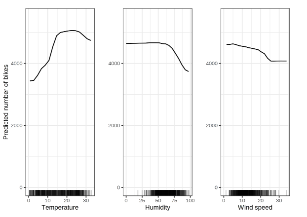As can be seen from the figure, the model predicts a large number of bicycles on average for warm, but not too hot weather, with more than 60 humidity reducing the desire to rent bicycles, and at the same time, wind speeds are largely completely negative, and wind speeds are higher and fewer people are riding.

Let's consider the PDF issue of a sorted variable and the impact of seasonal features on predicting bicycle rentals, as illustrated below. 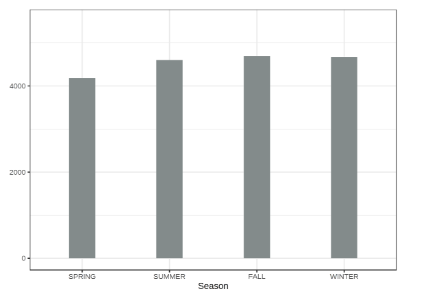We find that all seasons have similar impacts on model predictions, and in spring alone, models predict fewer bicycle leases. There's a difference between this figure and the graphics of the variance analysis, which only focuses on the average, and the variance analysis tends to use Boxplot to study the general distribution.

The PDP only takes into account the average and reasonable, because many models cannot output the difference estimates for regression.

We gave another example of a partial dependency that simultaneously visualizes both features, using colour maps as a method of distinguishing values and using some sort of discrete method of mapping. 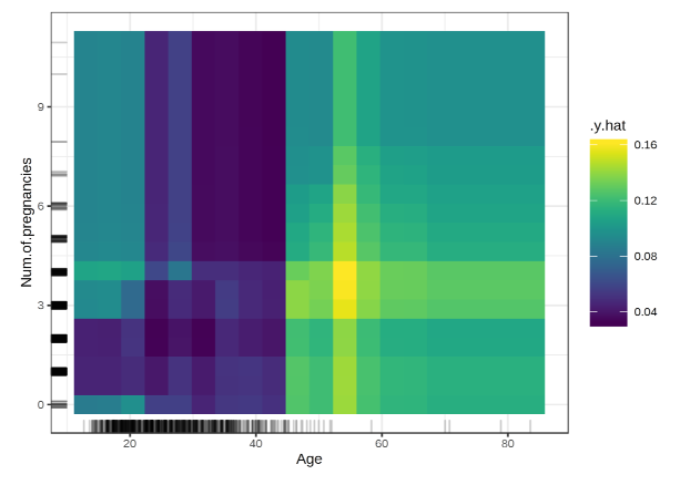It is easy to see that the greater the probabilistic value, the greater the Num, the larger the Age's bias.

Strengths

• Partly dependent on graphic calculations is intuitive and non-professionals usually quickly understand the PDP concept
• It's easy to explain the partial reliance on maps. It takes a simple reading ability and one or two examples to learn quickly.
• Part of it depends on the map.
• Partially dependent on chart calculations with causality

Disadvantages

• Partially dependent on actual in functionMaximum feature number is 2 This is because of the two-dimensional medium and our unimaginable high-dimensional space problem.
• Some PD charts do not show the distribution of features and strongly recommend using RUG (data point indicator on x axis) or histograms to help us understand the distribution of features. The PD map, which lacks characterizations, is likely to lead us to misinterpret some unprovoked predictions that have no samples.
• The assumption of independence is that PD's biggest problem, and we'll consider it later.
• The heterogeneity effects may be hidden because the PD curve shows only average marginal effects.

Heterogeneity: Assuming, for one feature, that half of your data point is positively relevant to the projection — the larger the feature, the larger the projection — the less the other half has negative relevance — the larger the projection. The PD curve may be a horizontal line, as the effects of the data set in two parts may be offset by each other. Then you can conclude that this feature has no impact on predictions.It's because some other variable is interacting., drawing an individual curve helps us find this problem

Individual expectations

Definitions

Individual conditions expectations (Individual Regulation, short ICE) displays a line for each example showing how the prediction of the example changes when the feature changes.

The characterization average effect relies in part on the map as a global approach, as it does not focus on specific examples, but on overall averages. PDPs with an equal value to a single data example are referred to as individual conditions expectations (ICEs) figures. PDP is the average of the ICE figure

All other features are the same, creating the variant of the example by replacing the feature with the value of the value in the grid and projecting these newly created examples using the Black Box model. The result is a set of features from the grid and corresponding predictions. Connecting it is what we want.

The purpose of ICE was to deal with the problem of partial reliance on maps that might mask an interaction-created isomer relationship, and ICE charts are more rational than PDPs when interaction exists.

The official definition of ICE is: $\begin{aligned}&\\text{in ICE {(x S^(i)}, x C^(i)}} {i}\text{in each instance, \hat{f} S^(i)}\text{is about}x S^(i)}\text{, at this time}x C^(i)}\text{&\text{changed. I'm sorry.

Example:

We also use examples to help us understand what ICE means and how to use the data set used in this paper for the "Culture Cancer Risks (Classification)" section of the model prediction that gives the probability of classification rather than the ICE graph 01. Icon 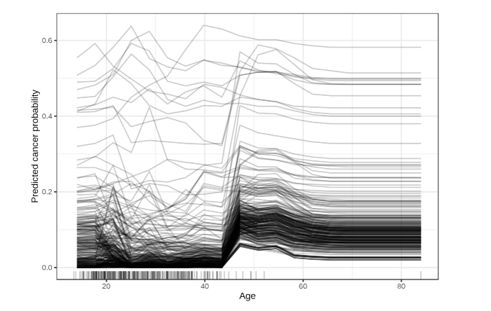It can be seen that the age effect follows the trend of average increase at age 50 (the trend for most people) and that for a small number of individuals who have a higher predictive probability at a young age, the predicted cancer probability will not change significantly with age. Basically following the same pattern, which means ICE and PDP basically reflect the same trend.

Strengths

Individual conditions expect curves to be more intuitive than partial reliance maps, and a line represents the projection of an example

ICE Curve reveals heterogeneity

Disadvantages

ICE curves can only show a meaningful feature, which is still due to the lack of plane media and human imagination.

If many ICE curves are drawn, the map may be too crowded to see anything, generalIt is suggested that some transparency be added and then superimposed。

It's hard to see averages in ICE drawings.Suggested mix with PDP

ICE can help us identify interactions, but it is still not possible to interpret them well, and if the characteristics of interest are linked to other features, some points in the line may be invalid data points

Cumulative Local Effects Chart

Thought

The cumulative local effect (Accumulated Local Effects Plot) describes how the average feature influences the prediction of machine learning models. The ALE figure is a faster, more unbiased alternative that relies partly on the PDP. Both approaches have the same goal.

We know that if the features of the machine learning model were relevant, then partial reliance would not be credible, and we actually produced some totally impractical samples in the PDP.$x_1$They can't exist in real applications, but we pretend everything's normal.

How do we get it?Estimation of characterization effects that respect identity relevanceWhat? We can average the condition distribution of the feature, which is$x_1$ , yes. $x_1$ Projections of similar examples are average. This method is called the Marginal Plot or M.

However, M-figures are not perfect, and M-figures avoid average predictions of data examples that are unlikely to occur, but they mix the effects of characteristics with those of all relevant characteristics. That is, even if a particular feature has no influence on the target itself, his relevance to an influential feature will be reflected in his influence.

So we bring out the ALE, which calculates the difference in projections rather than the average, based on the condition distribution of characteristics, that is,ALE charts how model predictions of data examples in this window are around $v$ Features $x_j$ A small "window" change

We use small windows to avoid the absorption of the relevant characteristic, which is essentially offset by the impact of that characteristic using differential techniques.

I don't usually use M-charts, so forget it now. Just remember, ALE does.

estimate

We just know the idea of the ALE, but we need a specific explanation of the way.

ALE for individual characteristics

First of all, we can calculate the uncentralized individual ALE. That's a good idea.{j,ALE}(x)=\sum\limits\(z k,j}\sum\lits i:x j^(i)}\j(k)}\left[f(z k,j},x {\(i)}-f(z k-1,j},x {\setminus})\ We know that ALE's idea is to calculate the difference in projections, so ours.$z$ It's a feature of real interest. We divide the compartments, and we finally calculate the average difference in the projection of this interval.

Centralize the effect. The average effect is zero. That's right.{j,ALE}(x)=\hat{\tilde{f}}{j,ALE}(x)-\frac{1}{n}\sum_{i=1}^{n}\hat{\tilde{f}}{j,ALE}(xThat's right. After centralisation, the ALE value can be interpreted as the main effect of the characteristic under a given value

The fractional number of the feature distribution is generally used as a grid for defining spacing. The use of fractional numbers ensures that an equal amount of data is available at each interval. The disadvantage of the fraction number is that the length of the interval may be very different. If the characteristics of interest are highly skewed (e.g., many low and only a few very high), this may lead to anomalies in some ALE maps.

ALE for the interaction of two features

ALE charts also show the interaction of two features. The principles of calculation are the same as individual features, but we use rectangular units instead of spacing. We omit the overly complex formula and use a chart to visualize it, as follows: 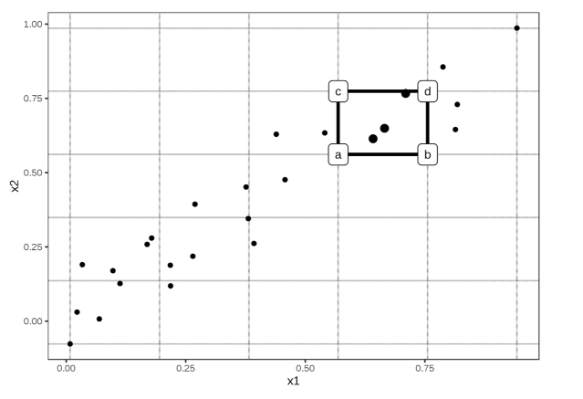We essentially need to calculate the second order of all examples within each grid cell. Bad

Since the ALE estimates for both characteristics show only the second-tier effects of the characteristics, particular attention needs to be paid to interpretation. The secondary effect is the additional interaction of the characteristics after consideration of the main effects of the characteristics.

It is assumed that the two features are not interactive, but each has linear effects on the projection results. In the one-dimensional ALE map of each feature, we will see a straight line as the estimated ALE curve.

But when we draw 2D ALE estimates, they should be close to zero, because the secondary effect is only an additional interaction. ALE and PD figures differ in this respect: PDP always shows total effects, ALE charts show first- or second-tier effects.

The ALE map of the classification features is complex and requires artificially defined distances, and we briefly present the analytical methods of the results when we encounter them, omitting theoretical descriptions.

Example:

We're still using examples to help us understand how the ALE diagram works, using the Bike Leasing (Return) part of the data set here to help us explain.

The use of ALE is generally limited to centralized ALE, and if we suspect the presence of characteristics, we should consider the use of ALE charts.

ALE based on temperature, humidity and wind speed prediction models

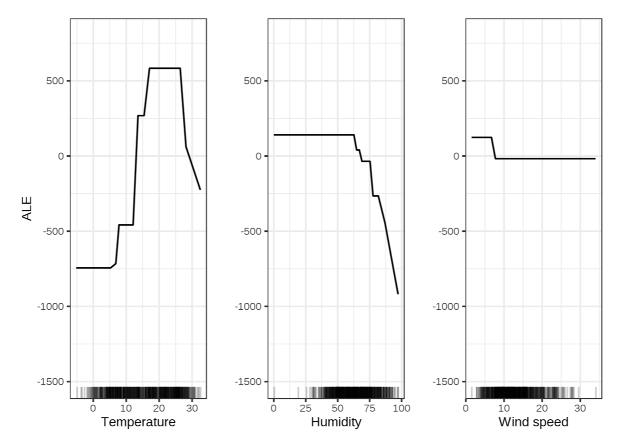
With regard to relevance, consideration of the relevant coefficient is the best option.

It's natural to read ALE and PDP.

The ALE chart of the classification variables is as follows: 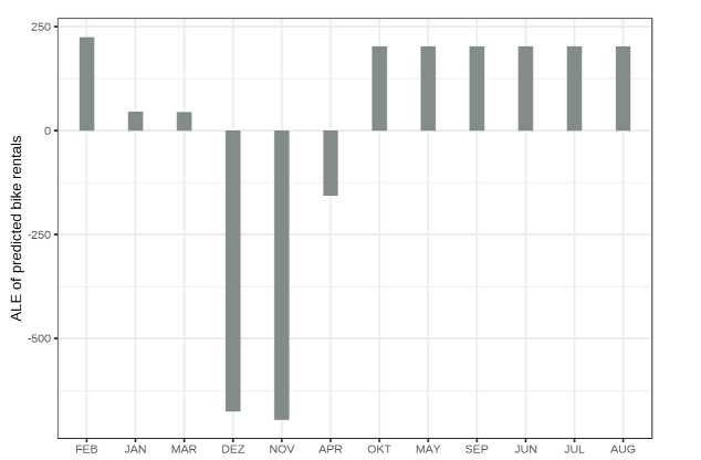We can give the same explanation as the PDP. It's just the ALE's centralization.

We consider the second-order effect of humidity and temperature on the projected number of leased bicycles, noting that he does not include the main effects, but only the issue of interaction. 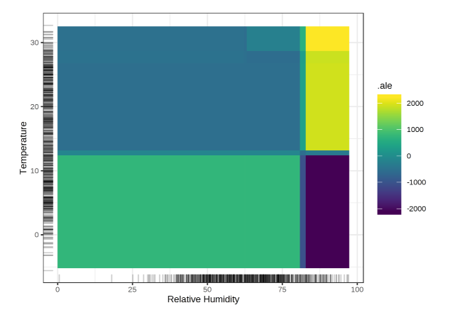You can see that hot and wet weather increases predictions. In cold and damp weather, it also has negative effects on the number of bicycles projected. Response

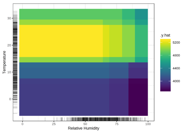
The main effects of humidity and temperature indicate that the number of bicycles is projected to decrease in very hot and humid weather. Therefore, in hot and humid weather, the combined effects of temperature and humidity are not the sum of the main effects, but are larger than the sum, and we may consider this time.Second-order PDP to reflect combined effects

Strengths

ALE charts are impartial, which means they remain valid when the characteristics are relevant. And the PDP is not valid.

ALE drawings are calculated faster than PDP

The interpretation of the ALE figure is clear: the relative impact of the change feature on the projection can be read from the ALE chart under the given value.

The ALE chart is centred on 0. That makes them better, because each point of the ALE curve is a difference from the average forecast.

2D ALE drawings show only interactive effects: if the two features are not interactive, they do not show anything.

In most cases, it is proposed to use the ALE figure instead of the PDP figure, as features are usually relevant to some extent.

Disadvantages

The ALE chart may become somewhat unstable (many small fluctuations, especially in the second-order ALE) and may be highly spaced, usually because of the problem of spacing setting, and the ALE chart may not be accurate if it is too small. If it's too large, the curve may become unstable.

ALE chart does not have ICE curves, does not deal with individual predictions, isthogenic.

It's a little annoying to explain the second-order effect map, because you always have to remember the main effects, which, like the PDP, make sense in the picture.

Even if the ALE chart does not deviate from the relevant characteristics,However, when characteristics are strongly relevant, interpretation remains difficult. We can't eliminate those effects.

Feature Interactive

Definitions

Characteristic Interaction: When the feature interacts in the predictive model, the projection cannot be expressed as the sum of the feature effects, since the effect of one feature depends on the value of the other. Aristotle's "whole is greater than the sum of the parts" applies where there are interactions.

The PDP is completely incapable of dealing with issues under the interaction, and ICE can allow us to observe the interaction from an intuitive perspective, but it is difficult to explain carefully that ALE has addressed the issue of characteristics and has explored some aspects of second-order interaction, which unfortunately are not sufficient.

We're working on PDP, ALE, ICE, and now we're working on it.

If the machine learning model projects on the basis of two characteristics, it can be broken down into four: constants, the first feature, the second feature and the interaction between the two. The interaction between the two features is the projected change by changing the characteristics after considering the effects of a single feature. The effect of the characteristics on the final projection is no longer independent.

One way to estimate the intensity of interaction is to measure the extent to which projected changes depend on the interaction of characteristics. This measure is called $H$ Statistics

Friedman's H Count

We will deal with two situations: first, using a two-way interactive measure, which tells us whether and to what extent the two characteristics of the model interact; and second, an overall interactive measure, which tells us whether and to what extent a feature interacts with all other features of the model.

If the two features are not interactive, we can split the partially dependent function as follows:Let's say the PDF's already centralized. $$PD_{jk}(x_j,x_k)=PD_j(x_j)+PD_k(x_k)$$ That is, the two-way partial reliance function of both characteristics is directly the sum of the function of the individual feature.

If a feature does not interact with any other feature, the entire predictive function can be broken down into the sum of the non-interactive and other characteristics that are partially dependent on the function as follows: $$\hat{f}(x)=PD_j(x_j)+PD_{-j}(x_{-j})$$

That's why we came up with the features. $j$and $k$ The interaction between the $H$ The statistics are: $$H_{jk}^{2}=\sum_{i=1}^{n}\left[PD_{jk}(x_{j}^{(i)},x_{k}^{(i)})-PD_{j}(x_{j}^{(i)})-PD_{k}(x_{k}^{(i)})\right]^{2}/\sum_{i=1}^{n}PD_{jk}^{2}(x_{j}^{(i)},x_{k}^{(i)})$$ The same applies to measurement features. $j$ Whether to interact with any other feature: $$H_{j}^{2}=\sum_{i=1}^{n}\left[\hat{f}(x^{(i)})-PD_{j}(x_{j}^{(i)})-PD_{-j}(x_{-j}^{(i)})\right]^{2}/\sum_{i=1}^{n}\hat{f}^{2}(x^{(i)})$$ If there is no interaction at all, the statistical amount is 0, if the interaction between the two features is counted as 1 means that each PD function is constant and the effect on the projection is only from interaction.

$H$ The assessment costs of statistics are high. $n$ Call required $n^2$ The prediction function at the secondary level can reduce performance costs by sampling the original data points, but can cause statistical instability.

Example:

Let's see what the interactive features are in practice, and we'll explain it in the context of the cycle lease (return) section of this paper, the risk factor for cervical cancer (classification) section of this paper.

We measure the interaction of the SVM model in the regression problem. 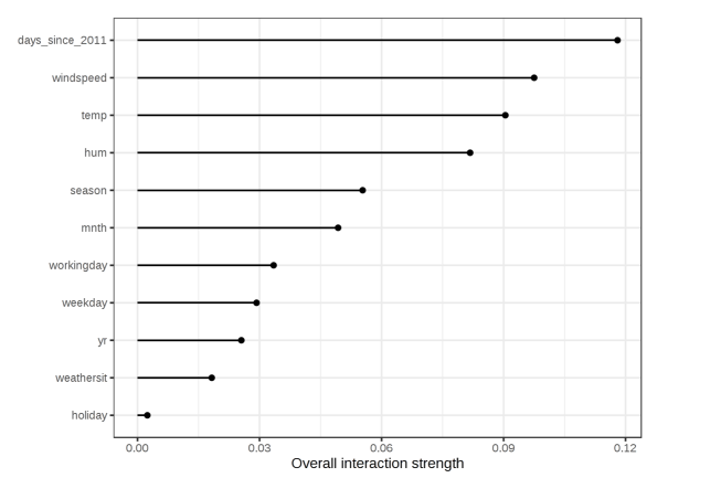Projections of the intensity of interaction of each characteristic of the support vector leased by bicycle with all other characteristics (H statistics) are shown in the figure above. Overall, interaction between features is weak (less than 10 per cent of the variance for each characteristic explanation).

Consider classification and use the RF model for prediction 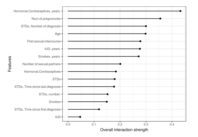A number of indicators, such as HC and NUM, are highly interactive. That's over 30 percent of the explanation.

After looking at the characteristics of each and all other characteristics, we can select one of them and then study in greater depth all the two-way interactions between the selected features and the other. Let's take the example of the NUM on classification. 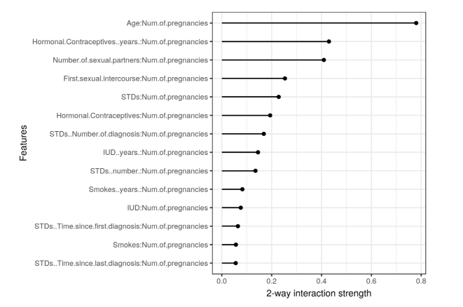This is the result of our analysis.

Strengths

Interaction $H$ Statistics are available through partial reliance on disaggregationTheory Foundation。

$H$ Statistically availableMeaningful explanation.: Interactivity is defined as the difference in shares explained by the interaction.

Because statistical information isUnspecified, and always between 0 and 1, so it is comparable between features and even models.

Statistical Information SocietyTest all types of interactionsWhatever their special form.

Use H stat, alsoYou can analyze any higher-level interaction., for example, the intensity of interaction between three or more features.

Disadvantages

Interactive H statistics take a long time to calculate because of itsIt's a big calculation.。

This calculation relates to estimated marginal distribution.If we don't use all the data points, there's a difference in these estimates.I don't know. This means that when we sample the points, the estimates also vary from operation to operation and the results may be unstable. I propose to repeat the calculations of H statistics several times to see if there are enough data to achieve stable results.

It's not possible to judge if the interaction is greater than zero, and there's no theory to help us deal with it, and it's hard to say when H's statistics are so big that we think the interaction is strong. Which means...It's all about experience.

Only the intensity of the interaction can be judged, and there is no capacity for more detailed analysis, which requires a return to 2D PDP or ICE analysis

Not applicable to computer visual problems because no image can be processed (in pixels)

It's too relevant to render the method ineffective.

Replace feature importance

Definitions

The replacement feature importance measures the increase in error in the model that we predict by replacing the feature value, which breaks the relationship between the feature and the real result.

The algorithms have the following ideas.

Training model$f$,Specific Matrix$X$ Target vector$y$, Error measure$L(y,f)$Estimated original model error$e^{orig}=$ $L(y,f(X))$ (e.g., average error) characteristics$j\leftarrow1$ to $p$By changing data$X$Characteristics in$j$Generate Feature Matrix$X^{perm}$。

It destroys the character.$j$And the real results.$y$The links are based on data replacement projections, estimated errors$e^{perm}=L(Y,f(X^{perm})$Calculate replacement feature importance$FI^j=e^{perm}/e^{orig}$I don't know. Alternatively, differences can be used:$FI^j=e^{perm}-e^{orig}$Sort features in descending order, in which comparable replacement feature importance is most common

Importance of using training data or testing data

At present, there is no complete answer to this question;

In the case of selection of training data, the combination seriously affects our correct thinking about the error in the model, resulting in the invalidity of the final character importance judgement;The importance of characterization based on training data leads us to mistakenly believe that characterization is important for prediction, whereas in fact models are simply oversyncs and not at all.

For the selection of test data: if all data are used to train the model, this means that there are no available test data, so we propose cross-validation to address this issue, but it means that the significance of the feature is calculated on a subset of the data expressed differently.

Therefore, if we choose the importance of training data computing features, it means that we want to know to what extent the model depends on each feature for prediction; and correspondingly, testing data means that we want to study the extent to which that feature contributes to the model ' s performance on unknown data.

We can't come to a definitive conclusion. We need more experience and research to help us think.

Example:

Characteristics of increasing model error to 1 times (= no change) It's not important to predict cervix cancer, and we're going to take the bike lease (return) section of this paper, the risk factor of cervix cancer (classification) section of this paper, and two data sets to discuss our problem.

For classification issues, 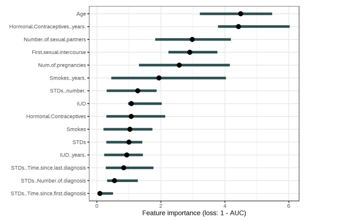There's something about return. 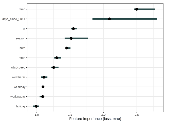There's basically nothing to explain.

Strengths

Good explanatory: Characteristic importance is the increase in model error when characteristic information is destroyed.

Between questions, the measure of characteristic importance is comparable (provided we use the margin)

The importance of changing features automatically takes into account all interactions with other features.

The replacement feature importance does not require a re-training model, which significantly reduces the operating costs

Disadvantages

We don't know whether to choose between training data or testing data to determine the importance of characteristics.

We need real samples, real and marked samples for training models.

If the features are relevant, the importance of changing the features may be biased by unrealistic data examples So it's still not going to be able to deal with the issue of strong relevance, and it's now the third model that can't be dealt with.

Global proxy model

Definitions

Now it's time to discuss proxy models, and we want to create an interpretable model that can train him to be close to black box predictions, and then deal with machine learning interpretability by interpreting proxy models.

Understanding proxy models does not actually require much theory. We want to be there. $g$ Explanatory constraints, proxy model prediction function $g$ Approach our black box prediction function as closely as possible $f$I don't know. For Functions $g$, can use the "explainable model" section of any paper

One way to measure the ability of the agent to copy the Black Box model is to use the R formula as $R^2=1-\frac{SSE}=1-\frac{sum *^{(i)}-\hat{y}^{(i)})^2}{\sumI don't know. And when online re-entry, we also looked at the R side, the R side of the linear re-entry base, where we mentioned that R had no true meaning, but with the proxy model,The R side can be explained by the percentage difference captured by the proxy model, which is the ability of the proxy model to explain the black box.

We don't talk about black box performance here, and if it's not good, then the proxy model's explanation becomes irrelevant.

The whole agency problem is training a new explanatory model. We don't waste time rereading it here.

Strengths

The proxy model is very flexible, so we can change the new black box model or replace the new interpretation model, and it's perfectly possible to hand it over to multiple teams in parallel.

Using R, we can easily measure the performance of our proxy model in approaching the black box prediction.

Disadvantages

The conclusion is that the model is not the data, since the proxy model will never see the actual results.

It's not clear what the R side's best cut-off point is, like the linear regression.

For a subset of a data set, it is explained that the model may be very close, while for another subset, it may vary considerably. In this case, the interpretation of simple models will vary for all data points. The local effects should therefore be considered.

All the strengths and weaknesses of the depreciable proxy model itself

Local proxy model LIME

Definitions

Local proxy models (Local interpretable model-agnostic models, LIME) are self-depreciable models forAn individual case prediction explaining the Black Box Machine Learning Model

The central idea of LIME is that for any complex black box model (Black-box Model), it is difficult to understand its decision-making boundaries from a global perspective, but it is possible to enter samples in a specific context.Local, a simple, self-articulated model (e.g. linear regression or decision tree) is used to approach and formulate black box models.

The model studied should be a good approximation of the local predictions of the machine learning model, but it is not necessarily a good global approximation, which is easier to approximate a local nature than the global approximation.

A mathematical explanation.

LIME aims to optimize the following target functions:

$$\xi(x) = \arg\min_{g \in G} \mathcal{L}(f, g, \pi_x) + \Omega(g)$$

• $x$: We need to explain specific input samples.
• $f$: Black box models to be explained (e.g. random forest, deep neural network).
• $g$: Explanatory model (usually simple model community) $G$, such as linear models).
• $\pi_x$: Local proximity measurement, defined in samples $x$ Weight of other nearby samples (range) $x$ The closer you get, the greater the weight.
• $\mathcal{L}(f, g, \pi_x)$: Solidity Loss, measured by $x$ It's a local neighborhood.$g$ Proposed $f$ Errors in forecast results.
• $\Omega(g)$: Complexity, we need to limit in order to ensure interpretativeity $g$ Complexity (e.g. limiting the number of non-zero characteristics of linear models).

Experimental and realization mechanisms:

1. Perturbation: Right Input $x$ Microturbation (e.g., in the case of text, some words are randomly discarded; in the case of images, some hyperpixel blocks are shielded) to generate new samples.
2. Black Box Forecast: Enter these new samples into the black box model $f$, obtain probabilities.
3. Weighted training: According to the disturbance sample and the original sample, $x$ Distance $\pi_x$ Calculate weights and then use these data to train one with regularity $\Omega(g)$ The White Box Model $g$。
4. Extract explanation: White Box Model $g$ the weight or structure of the $x$ Local interpretation of projected results.

Sample disturbance of data

We mentioned that LIME needed to create a data set based on an example of disturbance, and here we are presenting the method of disturbance.

For structured data, the basic disturbance is shown in the figure below. 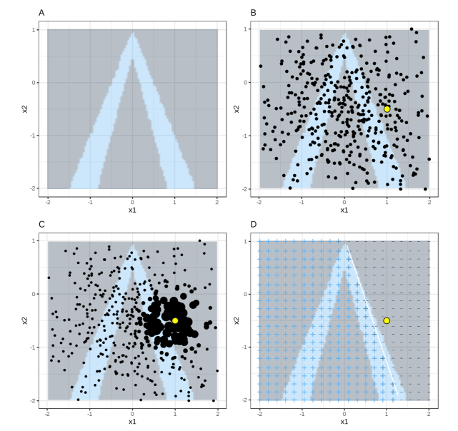The first is the original projection, the second is the point where some normal samples are generated in the case of interest, the third is the weight assigned to points based on distance and the fourth is the local learning method.

It is very difficult to define a meaningful neighbourhood around a point. The current LIME uses index smooth cores to define a neighbourhood, but there are many possibilities for nuclear parameter regulation, which will affect the outcome, but there is no defined way to help us determine it.

Here's one example: we use the feature effect: we multiply the weight by the actual feature value to judge the local effect of this feature.

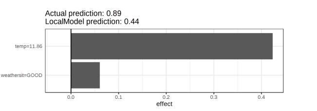
Strengths

Its advantages are broadly consistent with the global proxy model;

An explanation will be simple and effective when using LASO or a short decision tree.

Disadvantages

When using LIME for table format data, the correct definition of the neighbourhood is a large unresolved issue

SHAP: from methodological map to feature article

SHAP (SHAP) uses Shapley values to explain the characteristic contribution of a given projection to the baseline. It can provide partial attribution, and it can summarize the attributions of multiple samples into global importance, summary and dependency maps. TreeSHAP provides efficient algorithms for tree models, and KernelSHAP is calculated in a non-model manner.

It is appropriate to answer “why does the model give this prediction”, but it cannot be interpreted as a causal link to the real world. Both background data, feature relevance and the definition of “identity loss” change the outcome; the same model changes a sample of benchmarks, which may also be interpreted differently.

Full Shapley extrapolation, KernelSHAP, TreeSHAP, DeepSHAP, GradientSHAP, Background Data Selection and Project Errors were collatedShapley and SHAP - Model Explanatory SOTA ToolI don't know. There's no repetition here, just keeping SHAP on an interpretable map.

Sample-based interpretation

What's based on a sample explanation?

Sample-based Interpretations Select a specific example of a data set to explain the behaviour of a machine learning model or to explain the bottom data distribution, and he does not explain an example.

The explanation based on the sample is mostly unrelated to the model and the differences in methods not related to the model The reason is that the sample-based approach explains the model by selecting examples of datasets rather than by creating feature summaries (e.g., feature importance or partial dependence).

A sample-based interpretation would be meaningful only if we were able to present data examples in a way that humans could understand. This is very effective for the image.

Let's just give an example based on a sample.

A little cat sits on a window table in a fireless, uninhabited house. The fire department has arrived and one of the firefighters is considering whether he could venture into the building to save the kittens. He remembers what he met when he was a fireman.Similar situationThe old cabins, which had been burning slowly for some time, were often unstable and eventually collapsed.Because of the similarity of this situation,He decided not to enter because the risk of a house collapse was too high.

And that's what we want models to think like humans (at least at the level of interpretation): things like B, things like A, things A lead to Y, so I predict that B will also cause Y.

Counterfaction

Definitions

Counterfactual Interpretations describe a causal relationship in the following form: "Y would not have happened if X had not happened," thinking against facts requires conceiving a hypothetical reality that contradicts the observed facts, but rather the way humans think frequently.

The counterfact explanation of the model describes the smallest change in the characteristic value of changing the forecast to predefined output (anti-fact), i.e., if I wanted to change the fact that the loan was rejected, i.e., if I wanted to make an extra dollar a year, or if we wanted to raise the rent of our own house, we needed to expand the size of the house.

The counter-facts are human friendly interpretations because they contrast with current examples and because they are selective, which means that they usually focus on a small number of characterizations.

But the counterfact is beset by the "Roshenmon effect." The non-exclusiveness of a counter-fact interpretation deserves our separate consideration, and this multiple counter-fact problem can be resolved by reporting on all counter-fact explanations or by developing criteria to assess the counter-fact and choose the best counter-fact.

We usually ask for satisfaction.

• Counter-fact cases should produce predefined projections as closely as possible, i.e., do not change too many target values at once, such as classification probability and regression predictions. Value
• Counterfact should be as similar as possible to the examples of characteristic values so that as few features as possible can be changed Value
• Anti-facts cases should have possible characteristics, and there's no point in those counter-fact explanations that are completely out of step with reality.

Generate a counter-fact explanation

A simple way of producing counterfacts is to search through repeated experiments, but it's too stupid, so we usually use some methods of optimizing losses to generate counterfacts.

Wachter et al. recommend to minimize the following losses: $L(x,x)',y',\lambda)=\lambda\cdot(\hat{f}(x')-y')^2+d(x,x'That's it. The first is the square example of predictions and expected results, and the second is the distance between examples and counter-facts.$\lambda$ It's the coefficient used to mix the two effects, the larger it means we want to have the opposite facts closer to prediction, the smaller it means we want to change the characteristics as little as possible. Value

It's customary to use MAD's deformation as a distance behind. $d(x,x)')=\sum_{j=1}^p\frac{|x_j-x'_j|}{MAD_j}$$

As for the anti-fact example, it's very easy to understand.

Strengths

The explanations of the counterfacts are clear and very easy to understand.

An anti-fact approach does not require access to data or models. It only needs access to the predictive function of the model.

This method also applies to systems that do not learn by machine. We can create a counter-fact for receiving input and returning any system that is exported.

The counterfact interpretation method is relatively easy to achieve, as it is essentially a loss function that can be optimized using the standard optimized library.

Disadvantages

The counterfact interpretation method is relatively easy to achieve, as it is essentially a loss function that can be optimized using the standard optimized library.

Classification characteristics with many different levels cannot be well addressed. The authors of the methodology suggest that the method be operated separately for each combination of characteristic values of the classification characteristics, but if you have multiple classification features with multiple values, this will result in a combination explosion.

Fight the sample.

Definitions

Anti-sampling (Adversarial Express) is the case when a small change in a given characteristic value of a sample makes a miscalculation of the entire model. This is very similar to the counterfact explanation.The anti-sampling sample is an example of the opposite., designed to defraud models rather than to interpret models.

For example, machine-learning scanners are scanning luggage at the airport. To avoid detection, people invented a knife to make the system think it was an umbrella.

Methodology and examples

The approach in this section focuses on image taxonomyrs with deep nervous networks, where extensive research has been carried out, and visualization of anti-images has a strong educational significance.

The anti-image sample is an image with a deliberate disturbance pixel intended to defraud the model during its application. The samples are impressive evidence of how easily people can look at harmless images to deceive deep-seated nervous networks for target identification, and the changes predicted are not understandable to human observers. The anti-sampling samples are like optical illusions to machines.

Since the anti-smuggling sample is concentrated in the CV field, there are no more presentations here.

Examples of influence

The machine learning model is ultimately the product of training data, and the removal of one of the training examples may affect the model generated. When training examples are removed from training data, they change the parameters or projections of the model significantly, so we call this example “impacted”. By identifying examples of influential training, we can “debug” machine learning models and better explain their behaviour and predictions.

In this subsection, we do not view models as fixed models, but rather as functions of training data. Examples of influence can help us answer questions about global model behaviour and individual predictions.

Angular values and influential examples

An anomaly (also known as entanglement) is an example of other examples of distance from data concentration, and of impact when the anomaly impact model is used.

An example of impact is the example of data, whose deletion has a significant impact on training models. The greater the changes in model parameters or projections, the greater the impact of the example, when the model is retrained after the specific example is removed from the training data.

Delete Diagnosis

Examples of how the removal of the model has had a significant impact on the model are generally considered to have had an impact.

DFBETA assessed the coefficient shift after the deletion of an example. $$DFBETA_{i}=\beta-\beta^{(-i)}$$ Cook Distance can assess his impact on the overall predictive performance of the model, but only for the LM and GLM models, and the Cook Distance in a broad linear regression

The simplest impact levels for the model ' s projected impact can be written as: $$US$US$$US$US$$US$US$$US$$US$US$$US$US$$US$$$US$$US$$$$US$$$$US$$$$$$$$$$$$$$$$$$$$$$$$$$$$$$$$$$$$$$$$$$$$$$$$$$$$$$$$$$$$$$$$$$$$$$$$$$$$$$$$$$$$$$$$$$$$$$$$$$$$$$$$$$$$$$$$$$$$$$$$$$$$$$$$$$$$$$$$$$$$$$$$$$$$$$$$$$$$$$$$$$$...$$$$$$$$$$$$$$$$$$$$$$$$$$$$$$$$$$$$$$$$$$$${j}-\hat{y}\right|$$ It's a very common format.

Impact Functions

Sometimes we don't want to train so many models, especially when they're complicated.

So if there is a model with a loss function, the model's parameters have a second-ordered guide, we can consider using the Impact Functions to estimate the impact of the example on model parameters and projections.

The method of influencing functions requires a loss gradient associated with model parameters, which only applies to the subset of machine learning models, all of which are not tree-based, but the neural network is available, which is good news.

Strengths

The study of influential examples highlighted the role of training data in the learning process. This makes impact function and elimination of diagnosis one of the best debugging tools for machine learning models.

It's not a model to delete a diagnosis.

Disadvantages

The deletion of the calculation of the diagnosis is very expensive, as they require retraining. But the math is going to go way beyond what you think.

The impact function is a good alternative to deleting diagnosis, but only for micro-parameter models

The effect function is only similar, as it is expanded twice around the parameter. The approximation could be wrong.

There are no clear cut-off points for the impact intensity with or without impact

Impact intensity only considers the deletion of individual examples, not the deletion of multiple ones at a time. The group of data examples may have some interaction, but, in dealing with interaction, our computing needs are increasing exponentially.

Future

Prerequisites for forecasting

"Provision" based on three premises

• Digital: Any (interesting) information will be digitized
• Automation: A mission will be automated when it can be automated and when the cost of automation is lower than the cost of carrying out the mission over time.
• Incomplete target norms: We cannot perfect a limited target.

Digitalization is certain, automation will conflict with imperfect target norms, and it is therefore difficult for us to train a model that is completely automatic and perfectly achievable.

This conflict is partly mediated by means of interpretation.

A little story.

2030: Medical laboratory in Switzerland

"This is definitely not the worst way to die!" Tom concluded, "Trying to find something positive in this tragedy." He removed the pump from the IVF.

Lena added, "He died just for the wrong reasons."

"There are, of course, the wrong morphine pumps! They're adding to our workload!" Tom complained while he was pulling the backboard of the pump. After removing all the screws, he put the plate aside. He inserted the cable into the diagnostic port.

"You're not just complaining about work, are you?" Lena laughed.

“Of course not. Never!” He's sarcasm-bling.

He started the pump computer.

Lena inserts the other end of the cable into the tablet. "Okay, the diagnostic program is running." She said, "I'm really curious about what's going on."

"It did inject our John Doe into Nirvana. That morphine is very high. Dude, I mean... this is the first time, right? Usually, a bad pump only releases little sweetness or no taste. But never, like that crazy injection. Tom explains.

"I know. You don't have to convince me. Hey, look at that. Lena raised her tablet. "Do you see this peak? That's the efficacy of painkillers. Look! This line shows the reference level. This poor guy mixed multiple painkillers in his blood system that could kill him 17 times or more. Here's our pump injection. And then here she goes, "You can see here the moment the patient dies."

"Well, you know what happened, boss?" Tom asked his boss.

"Well... the sensors seem to be very good. Heart rate, oxygen level, glucose etc. Data collected as expected. There are missing values in blood oxygen data, but this is not unusual. Here, sensors also detect a reduction in heart rate and cortex levels caused by morphine derivatives and other painkillers. She continues to view the diagnosis.

Tom was obsessed with staring at the screen. This was his first investigation into the failure of the real equipment.

“Well, that's our first problem. The system failed to send a warning to the hospital's communication channel. The warning was triggered, but the emergency programme did not respond. It could be our fault, but it could be the hospital's fault. Please send the log to the IT team." Lena says to Tom.

Tom noded his head and his eyes were still on the screen.

Lena goes on to say, "It's weird. The warning should also lead to the shutdown of the pumps. But it clearly did not do so, and that must be a mistake. The quality team missed something. It's really bad. It may be related to the emergency programme.”

"So, somehow, the emergency system of the pump went down, but why was the pump so crazy and injected a lot of painkillers into John Doe?" Tom wondered.

“Good question. You're right. Apart from emergency emergencies, pumps should never have used that much medicine. Given the low level of cortical alcohol and other warning signals, the algorithm should have stopped earlier.” Lena explains.

"Maybe there's some misfortune, like a millionth of a millionth of a million?" Tom asked her.

"No, Tom. If you read the files I sent you, you'll know that the pump was tested first in animal experiments, then in humans.The perfect amount of painkillers is given by learning to input according to the sense. The pumping algorithm may be non-transparent and complex, but it is not random. This means that in the same circumstances the pump will again operate in exactly the same way and our patients will die again. The combination of the input or the unwanted interaction must have triggered the wrong act of the pump. That's why we have to dig deep to find out what's going on here." Lena explained.

"I understand..." Tom replied with a confused answer, "Isn't the patient dying soon? Because of cancer or something."

Lena noded in reading the analysis.

Tom, get up and go to the window. He looked out and looked at something far away. “Maybe the machine freed him from suffering and helped him to do him a favor and not suffer any more. Maybe it just did the right thing, like lightning, but, you know, a good lightning. I mean like lottery tickets, but not random. But for some reason. I would do the same thing if I were a pump."

She finally looked up at him.

He's been looking outside for something.

They were all silent for a moment.

Lena, keep your head down again and keep analysis. "No, Tom. It was a mistake. It was a fucking mistake."

Meaning of model interpretability

According to the previous story, we know that interpretability is an important point.When the results of the model have a major impact on the real worldThe major security problem of AI is very important at this time, and we do not want a black box model to cause enormous damage to society as a whole.

The blogger adds:When people need to interact with models, There is also value in explanatory, and more relevant studies may focus more on generating models than predictive models, which are discussed mainly in this chapter, and know why producing such results will guide us in adjusting the next generation to interpretive ones.

The future of machine learning.

The discussion explains the future of machine learning, and the future of machine learning.

• Machine learning will grow slowly and steadily.
• Machine learning drives a lot of things.
• Explanatory tools facilitate the introduction and research of machine learning

Explanatory future

• Emphasis will be placed on interpretive tools that are not relevant to the model
• Machine learning will be automated and interpretable.
• Data scientists will automate themselves and the program will interpret itself (same as the former).