Shapley and SHAP: State-of-the-Art Tools for Model Interpretability

This article is devoted to Shapley values and SHAP. If you need to understand the complete relationship between the interpretable model, the PDP, ALE, the replacement importance, LIME, the counterfact and impact function, you canExplanatory Machine Learning: Model Interpretation, SHAP and Anti-Factual MethodsStart.

The questions in this article can also be addressedExplanatory machine learning: model interpretation, SHAP and anti-fact methodsHow the concept of a relatively close read together is developed in different contexts.

Shapley Value, fair distribution of game theory.

Shapley values explain projections by assuming that each characteristic value of the example is the “player” in the game, where the projection target is total expenditure. Shapley values are a method of coalition games that will show us how to distribute total expenditures fairly among characteristics. We need to adopt a simple example of how to understand Shapley Valle from a theoretical point of view, so that it can be applied to the areas that are needed.

It is assumed that machine learning models have been trained to forecast apartment prices. For an apartment, the projected price is Euro300,000, which needs to be explained. The apartment is 50 square metres in size, located on the 2nd floor, near which there is a park, and where cats are prohibited from entering, the average forecast price for all apartments is Euro310,000. How much does each characteristic value contribute to the projection compared to the average projection?

We'll draw an analogy.

Game is a predictive task for a single example of a data set
“Proceeds” is the actual projection for this example less the average projection for all examples Value
" Player" is the characteristic value of the example

We want to use the player to explain the gain, that is, the characteristic value to explain the margin of 10,000.

Mathual definition of Shapley values: cooperative game model

In the game theory, a cooperative game is defined by two elements:$(N, v)$。

Players Gather (in %1)$N$): All players involved in the game. In your case, players are the characteristics. To clarify, we assume that this apartment has only three features:
- Player 1: Near Park
- Player 2: Ban Cats
- Player 3:50 m2 (Area)
  
  So, the total number of players $M = 3$Come on, men. $N = {1, 2, 3}$。
Feature Functions ($v$): Also called Value Functions, which represent any player's subset (Union) $S$The proceeds that can be obtained.
- In machine learning,$v(S)$ Defined as:In the subsets that only know $S$ Model expectations for housing prices in the case of medium-specific values。
- $v(\emptyset)$: The forecast value when there is no feature, i.e. the average price of all apartments (310,000 euros).
- $v(N)$: Final projection when all characteristics are present (Euro300,000).

Problem: We all have it. $v(N) - v(\emptyset) = -10,000$ “Failment” (total gain) for the euro. This - 10,000 euros, how exactly, uncontroversially, should be allocated to players 1, 2 and 3?

Dr. Shapley's answer in 1953, which is the first. $i$ Shapley value for a player (identity) $\phi_i$ The precise formulas are as follows:

$$ \phi_i = \sum_{S \subseteq N \setminus {i}} \frac{|S|! (M - |S| - 1)!}{M!} (v(S \cup {i}) - v(S)) $$

$S \subseteq N \setminus {i}$: means all players are not included $i$ The union (subset).
$v(S \cup {i}) - v(S)$: This is the player $i$ Join the Alliance $S$ And then I brought it.Marginal Contribution。
$\frac{\mid S \mid ! (M - \mid S\mid - 1)!}{M!}$: This is aWeight factorI'm sorry. It's the mathematical meaning of combining it: at all levels. $M!$ A possible player in order, player $i$ It's in the subset. $S$ , the number of the rows added immediately after the player has joined.

In summary:Shapley values are the average marginal contribution of the feature values in all possible alliances (Coalition).

Accurate calculation of the combination of house purchases

Now, we're going to calculate the Shapley value of "No Cat" ( Player 2) $\phi_2$。

Known $M = 3$, we need to build up all coalitions that do not include Player 2 $S$These are:$\emptyset$(Blank collection)${1}$、${3}$、${1, 3}$。

Assuming that we have obtained the following alliances by making the desired calculation of the data set: $v(S)$ Projected value (in EUR):

$v(\emptyset) = 31$
$v({1}) = 32$ ♪ Only the park ♪
$v({3}) = 30.5$ "Only 50 square meters."
$v({1, 3}) = 31.5$ ♪ Knows there's a park and 50 square meters ♪
$v({2}) = 30$ "Only a cat is forbidden."
$v({1, 2}) = 31$ (Park + no cats)
$v({2, 3}) = 29.5$ (Cats are forbidden + 50 m2)
$v({1, 2, 3}) = 30$ (All features are assembled, i.e. final projection)

According to the formula, we calculate the weighted sum of the four sub-items:

1. When $S = \emptyset$ (no feature exists, player 2 joins):

Weight:$\frac{0! (3 - 0 - 1)!}{3!} = \frac{2}{6} = \frac{1}{3}$
Marginal contributions:$v({2}) - v(\emptyset) = 30 - 31 = -1$
Weighted results:$\frac{1}{3} \times (-1) = -0.333$

2. When $S = {1}$ (Park features already exist, player 2 joins):

Weight:$\frac{1! (3 - 1 - 1)!}{3!} = \frac{1}{6}$
Marginal contributions:$v({1, 2}) - v({1}) = 31 - 32 = -1$
Weighted results:$\frac{1}{6} \times (-1) = -0.167$

3. When $S = {3}$ (50 m2 feature already exists, player 2 joins):

Weight:$\frac{1! (3 - 1 - 1)!}{3!} = \frac{1}{6}$
Marginal contributions:$v({2, 3}) - v({3}) = 29.5 - 30.5 = -1$
Weighted results:$\frac{1}{6} \times (-1) = -0.167$

4. When $S = {1, 3}$ (Parks and 50 m2 features exist, player 2 joins):

Weight:$\frac{2! (3 - 2 - 1)!}{3!} = \frac{2}{6} = \frac{1}{3}$
Marginal contributions:$v({1, 2, 3}) - v({1, 3}) = 30 - 31.5 = -1.5$
Weighted results:$\frac{1}{3} \times (-1.5) = -0.5$

Final calculation $\phi_2$：

$$ \phi_2 = (-0.333) + (-0.167) + (-0.167) + (-0.5) = -1.167 \text{ 万欧元} $$

ConclusionsThe feature, “No Cats”, strictly reduced the projected price of the house by 11,670 euros.

Value of Shapley Valle

You might ask: Why do you count with such weight? Just take the feature out and count the margin once. "that is, the idea of changing the importance of character, which is not perfect."

That is why Shapley's values are considered to be in the interpretable field.It's the only way to distribute the four following game justice simultaneously.

Validity (Efficacy / Addability)：

The sum of the Shapley values for all characteristics shall be precise equal to the difference between the final projection and the underlying value. There is no redundancy, no omission.$\sum_{i=1}^M \phi_i = v(N) - v(\emptyset)$
Symmetry：

If the two characteristics produce exactly the same marginal contribution in all possible alliances, then their Shapley value must be exactly equal. This ensures that algorithms are not biased against certain characteristics.
Virtual (Dummy Axiom / zero player)：

If a characteristic (such as a worthless gift from a house purchase) joins any alliance and joins any alliance, and the margin contribution is never zero, then its Shapley value must be zero.
Linear Group (Additivity)：

If we use Model A and Model B to forecast the house price separately, then add the results of both as the projection for Model C. Then a Shapley value for a feature in Model C is bound to be equal to the simple addition of Shapley values in A and B.

It's a problem.: In the face of machine learning models that include deep non-linear and interactive features, the traditional replacement feature importance (Permutation Importance) is difficult to address in terms of reliance and coupling between features. Shapley values give one by taking all possible "exit order" and taking expectations from all featuresA fairer way of attribution under the weight of the game theory.。

Apply examples

Characteristic Value $j$ The Shapley value is explained by the average projection of the data set. $j$ The value of a characteristic contributes to the prediction of this particular example by: $ϕ_j$ Shapley values apply to both classification (output probability) and regression issues.

We use the risk-based data set for cervical cancer as an example.

The data on cervical cancer is concentrated on the Shapley value of one woman. The projection is 0.57, which is 0.54 more than average probability. 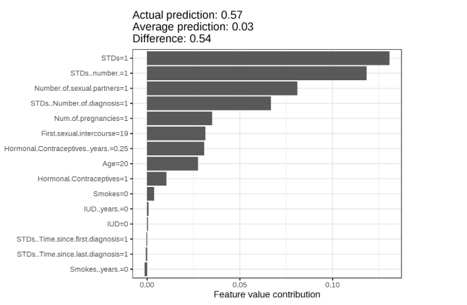And it's clear from this example that the impact of STDs is the greatest and the impact of increasing probability.

Shapley can achieve precise explanations for the comparison.

Shapley ValueAllows contrasting interpretationI'm sorry. Without comparing the projections with the average projections of the entire data set, you can compare them with subsets or even single data points. This introduces characteristics that are often overlooked by beginners in practical applications:Relativity of Interpretation。

In human cognitive habits, when we ask "why," we actually ask, "Why is A?" Not B?”. It's calledComparative InterpretationI'm sorry. We need to return to the feature function mentioned in the previous statement. $v(S)$ and base values $v(\emptyset)$。

Change background distribution (Background Distribution)

In the exact reasoning of the previous section, we set $v(\emptyset) = 310,000$ Euros. How did you get $310,000? It's a model in the context of our "no signature"Entire Data SetAll apartments are forecasted for price.Average。

Calculates the union value with some features $v(S)$ How do you deal with the mathematically when (for example, only “near the park”), those features of “not knowing” (for example, “area” and “does a cat have been allowed to be maintained” ?

The standard approach is to fill (marginalization) with the characterization values of other apartments in the entire data set, and then to expect. ** The actual meaning of this sentence is therefore:You can replace this "background data set to fill and calculate averages " , thereby changing the interpretation baseline (Baseline).

Let's use the example of apartments to practice these three contrast levels:

Compared with " Whole Data Set" (default standard scenario)

Background data100,000 apartments in the city.
Base Value $v(\emptyset)$Average city-wide housing cost: 310,000.
You're going to explain the problem."Why is this apartment 300 thousand?Average city-wideTen thousand dollars?
Meaning of the Shapley valueThe ban on cats (-11.67), near parks (+0.50) etc. is a contribution to the city-wide average.

Compare with "Specific Subsets" (comparable explanations - subsets)

Suppose you want to explain the price to a client who's looking at the old city. The average price for the city doesn't mean anything to him.

Background data: You only enter 5,000 apartments in the Old City as background data sets into the model.
Base Value $v(\emptyset)$Average housing price in the old city, assuming 350,000.
You're going to explain the problem."Why is this apartment 300 thousand?Average in the old city50 grand?
Meaning of the Shapley value: The Shapley values recalculated at this time will undergo dramatic changes. Because old city probably doesn't have parks in general, and this is the positive contribution of the "near park" feature. $\phi_1$ It'll be much bigger than before, and it fills the 50 grand gap between the average price of the old city.

Compare with " Single Data Point " (comparable explanation - individual)

That's the most extreme comparison. The client pointed to another apartment across the street (sold at 320,000) and asked you, "Why do I have a 300 million apartment on the same floor as the two rooms, in the same area?"

Background data: Only the “320,000 apartments” across the street are used as the only background data.
Base Value $v(\emptyset)$The estimated value of the contrast apartment (320,000).
You're going to explain the problem."Why is this apartment 300 thousand?The apartment across the street.Cheap, 20 grand?"
Meaning of the Shapley value: in this case, all the same features (area, segment) will be given a Shapley valueDirectly to 0(Because they do not differ between the two samples, the marginal contribution is 0). The final difference will be 100%, perfectly distributed to those who are not.Different features(e.g., a cat is allowed across the street, and the cat is forbidden.

Note that a comparative interpretation does not mean that the model will be retrained. The model is still being trained throughout the data set; in pursuing the explanatoryity that Shapley brings, we change the baseline for background data, thereby changing the interpretation baseline.

This comparison is useful in real business. The ability to customise benchmarks is also more difficult to achieve in a more stable way, such as LIME.

- We're gonna have to open the case."Why is the credit rating of user A lower than that of user B 50? " (Pilot data points compared)
Analysis of population disparities"Why is the probability of losing users this month 20% higher than the rate of active users last month?" (subset comparison)
Model Debug"Why is this negative sample miscalculated as positive scored so much higher than the real negative sample group?" (Subset comparison)

From the change of shaP calculation background_data Parameters (Python Extension) can transform model interpretation from general to precise impact. Shapley's excellent and interpretable skills are one of the best ways to do it.

Advantages and disadvantages

As can be seen from the above extrapolation, the complexity of calculating the Shapley value is that $O(2^M)$I'm sorry. If the model had 100 features, even using the world ' s top super-calculation would be the exact value of a prediction before the destruction of the universe. This is why the purely theoretical Shapley values “cannot be widely applied” in machine learning until the SHAP technology appears.

Shapley values may be misunderstood. The Shapley value of the feature value is not the difference in the projection after the feature has been removed from the model training. Shapley values are explained by the current set of feature values, which contribute to the difference between the actual and average projection values, which are estimated Shapley values.

The explanation created using the Shapley value method always uses all features. It's not appropriate for people who seek a thin explanation.

Shapley values return a simple value for each feature, but no predictive model like LIME

SHAP - Faster, more usable

From theoretically perfect Shapley values to engineering-based SHAP (SHAP) is a leap in the field of interpretativeity of machine learning. To understand SHAP, it cannot be seen as a Python library. And what is more important is:What were the flaws in the Shapley values that Lundberg and Lee had addressed when they introduced SHAP in 2017? What's the compromise?

Dimensions disaster and approximation calculations

We have extrapolated in the previous section that calculating the exact Shapley values requires all possible combinations of features, the time complexity of which is, $O(2^M)$I'm sorry. For a model with 100 features, even a sample would take a terrible time and would be totally unrealistic.

How did SHAP work out? SHAP did not invent new distribution theory, but cleverly converted the Shapley value into a single one.Addive Special Characterisation Method (Additive Special Organization Method)I'm sorry. It introduced a simplified local interpretation model. $g$：

$$ g(z') = \phi_0 + \sum_{j=1}^M \phi_j z'_j $$

of which $z' \in {0, 1}^M$ 表示特征是否存在的二进制向量（1 表示特征在联盟中，0 表示被隐藏），$\phi j$ is the Shapley value we're counting.

To solve this equation, SHAP has proposed two main approximation algorithms:

KernelSHAP (memode unrelated)：

It's a...Weighted linear regressionI'm sorry. It randomly extracts a portion of the union $z'And assign a weight to each union -Shapley Kernel $\pi_{x'}(z')$：

$$ \pi_{x'}(z') = \frac{M - 1}{\binom{M}{|z'|} |z'| (M - |z'|)} $$

Ration factor obtained by minimizing weighted square loss to match linear models $\phi_j$ The nearest Shapley value. This directly integrates the LIME and Shapley values in mathematics.
TreeSHAP (street model specific)：

Using the internal structure of the decision tree (separate paths and sample coverage of nodes), the complexity of calculation is reduced from index to multiple Level $O(TLD^2)$（$T$ For the number of trees,$L$ For leaves,$D$ For depth. That's why SHAP would be so quick in XGboost or LightGBM.

The problem seems to have been solved, but this approximation means we must have lost something.

What exactly does the "missing" of the features mean? (The Missingness Problem)

In game theory, the absence of a player is easy to understand (he does not participate in games). But in machine learning, the absence of characteristics is a very controversial mathematical issue. Once your model is trained, you must eat all the features, and most models cannot enter one directly into the nervous network. NaN。

The choice and discussion of SHAP:

To calculate the union value of the component features $v(S)$, we need to be able to read the features that are not in the alliance. $\bar{S}$It's a process. There are two distinct paths in the academic world:

Marginal Expectations (Marginal Exportation/ Intervention)：

Force break-up of the connection between the features, assuming known features $X_S$ and unknown features $X_{\bar{S}}$ Be independent. The practical operation is to randomly replace missing features with values in the Background Data.

$$ v(S) = E[f(X_S, X_{\bar{S}}) \mid X_S = x_S] \approx \int f(x_S, X_{\bar{S}}) dP(X_{\bar{S}}) $$

Problem: This can lead to seriousAnti-fact samples (out-of-distribution, OOD)I'm sorry. For example, the Alliance retains “pregnancy = True” but has filled “gender = man” with background data, and the model is forced to predict a data point that is completely unrealistic. This is the area where the shap has been sorely ill.
Conditional Expectations (Conditions Export / Observation)：

Considering the correlation between features, extrapolation of unknown features from a distribution that meets the conditions of known features.

$$ v(S) = E[f(X_S, X_{\bar{S}}) \mid X_S = x_S] = \int f(x_S, X_{\bar{S}}) dP(X_{\bar{S}} \mid X_S = x_S) $$

Problem: it contradicts the "virtual justice" of the Shapley values. If the model is not used at all for feature A, but the characteristic A is strongly associated with feature B, the condition distribution will wrongly attribute part of the credit for feature B to feature A.

Current status: Standard shap The library defaults to use the first type (marginal expectations/background data replacement), as it is easier to calculate and meets the instincts of causal intervention, but this raises the next fatal question.

Characteristic Relevance Trap (The Correlation Trap)

This is one of the most difficult research challenges in the AI field that can be explained at this time, and because the marginal expectation method produces unreliable samples, it leads to distortions in the final calculation of SAP Value, and only because of the relevance that will appear in high-dimensional statistics.

An extreme example is the assumption that “house area (m2)” and “house area (m2)” are thrown into the model at the same time. Because they're 100% relevant, the model actually needs only one of them to make perfect predictions.

If TreeSHAP is used, it may randomly assign weights on both of these features (e.g. 50% on one side). This could have led to an otherwise critical “area” feature, which had been reduced in importance and fell sharply in the SHAP summary.
This would mislead the operatives and make them think that the area is not important.
The consolidation of highly relevant indicators was necessary, but could not fully address the problem.

The directions worth studying.: The academic community is now studying the imposition of the order of interpretation of characteristics by calculating “asymmetric Shapley values” or by combining “causal Graphics” to strip off mixed co-linear interference.

Relevance vs. causality (Correlation vs. Causation)

This is a common area of error in thinking when applying SHAP, and in causal and ex post facto interpretation.

SHAP explains ** "What patterns models learn.", not“What is the causal link in the real world”**.

If your model finds that the lighter is highly likely to cause lung cancer, SHAP will honestly tell you that the characteristic of the lighter is a very positive contribution to increasing the disease prediction.

But in operational applications, if you conclude that “the confiscation of people's lighters can reduce the incidence of lung cancer”, it is a big mistake. SHAP is only a faithful reflection of the bias of the model and its relevance in the data, and it cannot replace causal inference.

Example:

Below is an overview of the organization of SHAP syndication interpretation, feature importance, summary diagrams, reliance on maps and interactive values, which is based on the following: Interpretable Machine Learning .

We'll use the risk factors of cervical cancer as examples of a disaggregated data set.

Because SHAP calculates the Shapley value, the explanation is the same as in the Shapley Example section, although we have some interesting visualizations as follows: 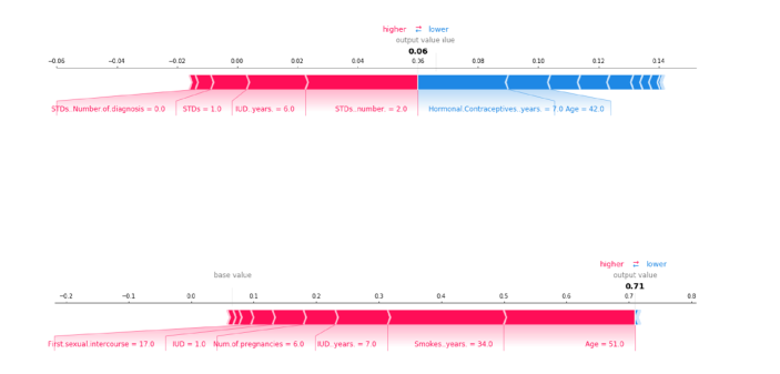The arrow and length reflect the SHAP effect with the position of the median line. Reactions

The first example, though STDs have increased the probability, was filled with a lot of retrofitting.
The second example is because Age and other factors increase probability, and eventually there's a lot of probability. These are explanations of individual projections.

Shapley values can be combined into global explanations. If we run SHAP for each instance, you will get the Shapley value matrix. This matrix has a row for each data instance and a column for each feature. We can interpret the entire model by analysing the Shapley values in this matrix.

SHAP Characteristic Importance

The idea behind the importance of the SHAP feature is straightforward: the larger Shapley absolute value is more important. Because of the global importance we need, the absolute Shapley value for each feature is averaged in the data:

$$ I_j=\sum_{i=1}^n|\phi_j^{(i)}| $$

We can map the importance of the SHAP feature.

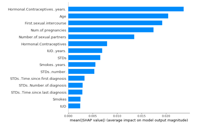
SHAP Characteristic Importance is an alternative to the importance of changing features. There are significant differences between the two measures of importance: the importance of the replacement feature is based on the decline in model performance. SHAP is based on the size of the characteristic attribution.

SHAP Summary Chart

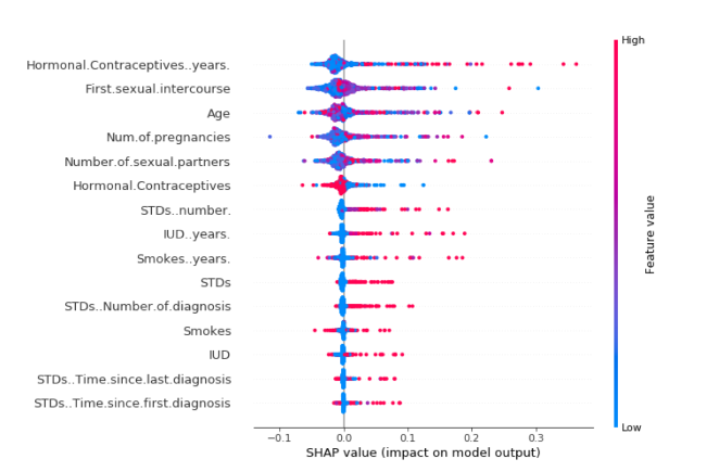
The feature importance map is useful but does not contain information other than materiality. To obtain more information, use summary charts

The summary chart combines the importance of the features with the effects of the features. Each point in the summary is a feature and an example of a Shapley value. The position on the y-axis is determined by the feature and the position on the x-axis by the Shapley value. These characteristics are sorted according to their importance.

SHAP dependency diagram

In the summary, we first see the relationship between the value of the feature and the impact on the projections. But to know the exact form of this relationship, we have to look at the SAP dependency map.

SHAP Character Dependence is probably the simplest global interpretation: mathematically, he's just the following scattered point. Figure

$$ {(x_{j}^{(i)},\phi_{j}^{(i)})}_{i=1}^{n} $$

As shown in the figure below: 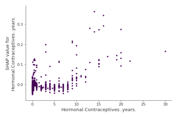As can be seen, the increase in HCyears increases the SAP value; it increases the probability of disease significantly.

SHAP Dependency Charts are an alternative method that relies partly on the charts and cumulative local effect maps, not on average but on the assessment of the global effect. SHAP$y$The fragmentation of the axis tends to imply the existence of interaction.

SHAP Interactive Value

The interaction effect is the additional combination of characteristics after considering the individual characteristic effects. Shapley Interactive Index Definition in the Game:

$$ \phi_{i,j}=\sum\limits_{S\subseteq\setminus{i,j}}\frac{|S|!(M-|S|-2)!}{2(M-1)!}\delta_{ij}(S) $$

The SHAP dependency figure that takes into account an interactive feature is 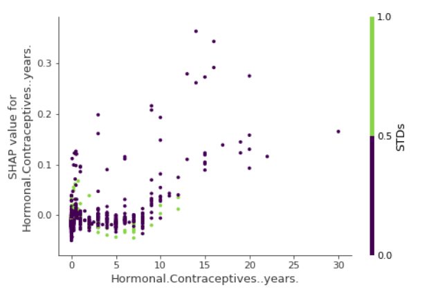High STDs lowers the last SHAP value

Depth extension of SHAP: black box decomposition of the nervous network

When processing table data, TreeshaP solves the problem of interpretation of tree models represented by LightGBM or CatBoost, by their time complexity at multiple levels. But in the real algorithm evolution, when we face deep learning structures that contain dense and thin features (e.g. DeepFM, Twin Towers or Large Language Models), Treeshap is powerless, and KernelSHAP ' s calculation costs are expected to trigger a significant explosion as the depth of the nervous network increases.

To address the attribution of the characteristics of the deep learning model, the academic community has extended two sets of specialized approximation frameworks:

DeepSHAP: A trans-chain based on reverse transmission

DeepSHAP is a suitable version of DeepLift algorithms. It's about:The contributions are distributed by using the Backpropagation mechanism of the nervous network, which bypasses violence.

The rationale.: DeepSHAP requires a " Background input " and an " Actual input " . When the data is moving through the network, the margin of each neuroactive value is recorded (in the case of a single neuron)$\Delta y$) and the input margin ($\Delta x$）。
Linear approximation: For non-linear activation functions (e. g. ReLU or Sigmoid), DeepSHAP calculates a 'multiplier 'by linear interpolation values $m_{\Delta x \rightarrow \Delta y} = \frac{\Delta y}{\Delta x}$。
Chain Law Reverse: From the output layer onwards, the variation in the output projection is transmitted in reverse by the lateral transfer using the revised chain rule until the input layer. The gradient that eventually falls on each input feature accumulates is the approximation of the Shapley value of that feature.

Gradient SHAP: aspirationalization of the gradient

GradientSHAP combines the theory of game between the Integrated Gradients and SHAP, especially for the continuous Embeding vector space.

Maths Essentials: It assumes continuous change in characteristics. Calculates the gradient of the model output relative to the input on these points by adding multiple random linear interpolation values to the Gaussian Noise between the background distribution and the current input.
Formula Thinking: The feature's SHAP value is approximated as its fraction of the gradient above the plug-in path:

$$ \phi_j \approx (x_j - x'_j) \int_0^1 \frac{\partial f(x' + \alpha(x - x'))}{\partial x_j} d\alpha $$
Apply sceneAnd when you need to explain what the high-dimensional Embeding captured, or when smoothing the sharp gradients that are generated by models that are not linear, GradientSHAP is a very powerful theoretical weapon.

Project Guide for SHAP

In real-life industrial applications, SHAP is by no means just a tool for generating reporting charts after model training has ended. It can be embedded in the pre-frontal feature engineering conduit as a data-processing tool.

Compression of Background Data (K-Means approximation)

The edge expectations in the formula require us to enter a background data set when calculating KernelSHAP or DeepSHAP.

A trap.: direct input of hundreds of thousands of lines of training as background data shap.DeepExplainerI'm sorry. This would allow the model to calculate expectations hundreds of thousands of forward reasoning for each sample, which would immediately cause the Out Of Memoory (OOM) collapse.
Engineering: At the code level, the background data must be down-dipped. The standard practice is to use K-Means cluster, which consolidates large-scale training into dozens of representative physiocentrics.

This, while retaining the overall margin distribution of the data, reduces the complexity of the calculation by several orders of magnitude, which is the engineering compromise available under SHAP for big data. And this background data itself is at the heart of our study of the exact interpretation of comparison.

Insisting massive data cleansing

A solid data base is the lifeline of subsequent model fine-tuning or enhanced learning. SHAP is an extremely efficient abnormality check.

Data Leakage Detection：

In the SHAP Summary (Summary Plot), if a characteristic that should be flat, its SHAP absolute value is a leading example of a cliff breaker and perfectly dominates the classification. This usually means that data leaks occur (e.g., inadvertently characterizing the “last login time” to predict whether there is a “loss”.
Offset Points and Scanning of Dirty Data：

In the SHAP dependency diagram, the normal feature distribution creates a clear non-linear curve or step leap. If an isolated dispersing point is present at the extreme position of the X axis and its SHAP effect (Y axis) is completely contrary to business commons, this strongly suggests that the characteristics of the sample are dirty data at the pre-processing or fusion stage. It is important at this point to return immediately to the early large-scale data cleansing logic to add cut-off or filter rules.

Dealing with co-linear engineering compromises (feature grouping)

To address the " character relevance trap " , asymmetrical Shapley values at the purely academic level are too costly to calculate when highly relevant features (such as multiple dimensions of user activity indicators) have to be fed to the model.

Engineering: At the interpretation stage, not a single SHAP value for a single feature, but rather a " Feature Group " wrapping of the strong competitor linear feature at the code level. Only the contribution of this Group as a whole Shapley value value is calculated. This would prevent the misallocation of importance and ensure that the global added value of justice is not undermined.

References

Christoph Molnar, Interpretable Machine Learning: A Guide for Making Black Box Models Explainable, 3rd ed., 2025. Official Page
Christoph Molnar, “SHAP” chapter, Interpretable Machine Learning. Chapter Link
Scott M. Lundberg and Su-In Lee, A Unified Approach to Interpreting Model Predictions, NeurIPS 2017. NeuIPS Page
Lloyd S. Shapley, A Value for n-Person Games, 1953.