Nonlinear Regression: Intrinsic Nonlinearity, Polynomial Models, and Nonlinear Least Squares

Non-linear regression

We know that some non-linear models can be converted into linear regression models by some transformations, which we call internal online; some models cannot be converted to linear models, and no matter how they are, we call them internal non-linear models, and we introduce them separately.

Internal online model

Multiple Returns

Multi-form regression is the most classic inlinear model; we'll only introduce one-dollar multi-linear regression models in the form of the following: $$y_i=\beta_0+\beta_1x_i+\beta_2x_i^2+\cdots+\beta_kx_i^k+\varepsilon_i,\quad i=1,2,\cdots,n$$ It's easy to know.

Multiple-transactional Returns

Multiple returns have a problem, number of times$k$When it was older. $x,x^2...x^k$The proximity of linear correlations, which can cause a great deal of difficulty in solving the normal equation, leads to a greater computational error; the corresponding difference is the difference between the equations we estimate, so we introduced the active multi-turning model. $$y_i=\beta_0+\beta_1\varphi_1(x_i)+\beta_2\varphi_2(x_i)+\cdots+\beta_k\varphi_k(x_i)+\varepsilon_i,\quad i=1,2,\cdots,n,$$ of which $$0$begin=0=\vvvv==================================================================================================================================================================================================================================================&j=1,2,\cdots,k,\\\sum_{i=1}^n\varphi_j(x_i)\varphi_q(x_i)=0,&\neq=1,2,\cdots, k.end{cases} We don't give a specific extrapolation formula.

Inlinear nonlinear regression

We'll use only the non-linear minimum two-fold and very large-like models. Model as $$Y=f(X_1,X_2,\cdots,X_p,\theta_1,\theta_2,\cdots,\theta_k)+\varepsilon,$$ We can use a very seemingly nuanced approach to squared and minimized the difference, which is, $$\min\quad Q(\theta)=\sum_{i=1}^n\left(y_i-f(X^{(i)},\theta)\right)^2.$$ The exact method of calculation is not pushed to the point where R provides the corresponding function, which involves the optimal question.

The questions in this article can also be addressedLinear regression base: linear model, minimum 2x2 estimate and regression diagnosis、Logistic regression: 2-classic because of variables, linear probabilities model and Logit modelHow the concept of a relatively close read together is developed in different contexts.

The median coefficient for the non-linear regression model is not as intuitive as linear regression, and we would be better advised to explain a regression model by drawing or tabulating changes in target variables when they change, regardless of the formula, which should be the same for the logarithmic transformation regression model.

Some ideas for a disability analysis.

Now we've probably understood the meaning of disability, and we can use it to try to deal with the real problem. According to the proposal, if we create a cross-reference to the proposed value vector,$\hat{y}$ The vertical axis is the student disability.$r_{i}$The difference between the two is that the point on the plane should be roughly evenly set in a horizontal zone. Internal 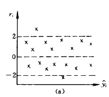This is a picture that means we're assuming.$e\sim N(0,\sigma^2I)$ It's basically reasonable.

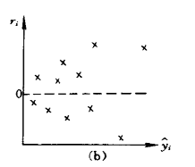
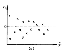
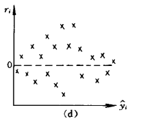These three pieces of the gap figure mean that the error and the difference are not valid. 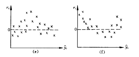Both of these means that our assumptions are problematic, and it's probably a non-linear model, which can be a very large cause of the disability analysis, which requires experience to address. And of course, we can also create other disability analysis maps, like research disabilities over time, based on a self-variant, and so on, and disability analysis is a very important part of regression diagnosis, and we're not doing enough here. The problem with disability analysis needs to be addressed gradually. For example, if you think you lack a retrogressive item, you can start a transformation to make it linear when you think it's non-linear. In case of error differentials, you can use a variation like Box-Cox (choose to change to high freedom) and apply a weighted minimum two-fold estimate, etc. The disability analysis is not just a small part of what we're presenting here, but we'll learn more about disability analysis later, but not now. The most common disability analysis is histograms to analyze the disability normality, QQ to analyze the disability normality, SW to test the normality of the disease, travel to analyse the independence of the anomaly, etc.

The disability is determined by the relevant judgment. The treatment is GLS technologies like Cochrane Orcutt and Prais-Winsten.

Add lags to the model for example we could specify an autoregressive distributed lag (ARDL) model

Leave model alone but fix the standard errors using Newey-West/HAC standard error

There's no detail here. There's a chance to add.

Hartley Test (Hartley)'s F-max Test)

Formula:

$$ F_{\text{max}} = \frac{\max(s_1^2, \dots, s_k^2)}{\min(s_1^2, \dots, s_k^2)} $$

Meaning: Calculates the margin between the maximum and the minimum values for the difference in the sample range of each group.
Conditions of application: Requires equal size of the sample groups (balanced design).
Original assumption (H0): The overall variance is equal for all groups ($\sigma_1^2 = \sigma_2^2 = \dots = \sigma_k^2$）。
Deny Field: When $F_{\text{max}}$ When the threshold is exceeded, the original assumption is rejected as not having been the same.

Cochran Test (Cochran)'s C Test)

Formula:

$$ G = \frac{\max(s_1^2, \dots, s_k^2)}{\sum_{i=1}^{k} s_i^2} $$

Meaning: Calculated the maximum sample variance as a proportion of the sum of all sample differences.
Conditions of application: Same requirement for the groups of samples.
Original assumption (H0): The overall variance of all groups is equal.
Deny Field: When $G$ When the threshold is exceeded, the original assumption is rejected as having a significant bias.

Bartlett Test (Bartlett)'s Test)

Formula:

$$ \chi^2 = \frac{1}{c} \left[ \sum f_i \ln s_i^2 - f_e \ln s_e^2 \right] \sim \chi_{k-1}^2 $$

Meaning: Based on the amount of the calculator that is constructed with a logarithmic value, the difference in the total of multiple normal distributions is tested as equal.
Conditions of application: Data need to be near-normal; not-normally-sensitive.
of which：
- $f_i = n_i - 1$ It's the first. $i$ Freedom of group (%1)$n_i$ As No. $i$ Group sample volume)
- $s_i^2$ It's the first. $i$ Sample differences for group
- $f_e = \sum f_i$ It's total freedom.
- $s_e^2 = \frac{\sum f_i s_i^2}{f_e}$ is the merger difference (weighted average difference)
- $c = 1 + \frac{1}{3(k-1)} \left( \sum \frac{1}{f_i} - \frac{1}{f_e} \right)$ is the correction factor (for small sample correction)
Original assumption (H0): The overall variance of all groups is equal.
Deny Field: When $\chi^2$ Value greater than $\chi_{k-1}^2$ When the top-side fraction of the distribution is selected, the original assumption is rejected.

00:43. The difference is the difference between the data to be compiled and the real data to be studied, and the appropriate display and study of the difference can draw attention to certain pre-neglected systemic behaviours in the data.

Research disability

Data is a superseding of the composition and the residuals, and we want to keep analysing the residuals and revise our proposeds.

The way back functions are used may be wrong, and we're thinking about the pattern from the disability analysis. Some informal criteria are: no pattern in the disability, all caused by random error, smaller margin squared, better proposed advantager r

We often use the assumption of disability in mathematical statistics, where this well-defined distribution of disability is best used to achieve the desired alignment, and vice versa to examine whether the proposed margin is consistent with the assumption, the most important of which is the study of the disability map.

A more classic residual analysis is an off-group site test.

So long as we use a robust method of extreme tolerance, the model will largely ignore the presence of the discrete points, and the residual analysis will be a good way of exposing the presence of the disempowerment points.

The difference in calculations is a complete set of data that we can continue to put into the analysis of eda, do what we do in the description statistics, study distribution, concentration separation, shape, etc.

Most of our methods of alignment tend to minimize a function of the disability, like Les, when we study the pattern of the disability, we can change functions like the weighted disability squared and the difference of the difference of the difference.

Restrictive cube

In scientific research, we often construct regression models to analyse the relationship between variables and variables. A major assumption of most regression models is that the variables are linearly related.

When there are non-linear relationships, we need to use some non-linear means of return. For example, multiple regression methods or the question of converting a continuous variable into an discrete variable for classification.

Unfortunately, the direct construction of multiple returns may have problems of overcompatibility, co-linearity and so forth. Dispersion factors can result in loss of part of the information and the location of nodes is more complex than the choice of categories.

I'm not sure."Restricted cubes."One of the most common methods of analysing non-linear relationships is the RCS.

The stylist (spline) is originally a flexible piece of wood or metal used to draw smooth curves.The root of a bar curve is a multi-segment function, this function is limited to certain control points and is called ""Nodes, the type of the line curve is determined by the number and location of the nodes, the multiple types, and the number and location of nodes.Cubeis the function of a three-time polygon.Limitsis an additional requirement based on the regression of the sample: the sample function is in two compartments at both ends of the variable data range [X1,X2) and (Xn-1,Xn] is a linear function.

The above presentation allows us to understand what the Cube is about, he is just a non-linear way of returning.

The number of RCS nodes is more important than location.I'm sorry. Because the choice of nodes is related to freedom, more nodes can be taken when the sample is larger. But the more nodes, the more freedom, the more complex models, the harder to solve.

It is suggested that the number of nodes be 4 and that the proposed effect of the model be better, i.e., it is possible to balance the smoothness of the curve and avoid the reduction of precision caused by over-choice. When the sample is larger, five nodes are a better option. Small sample ($n)<30) you can choose three nodes. When the number of nodes is 2 the condensed curve is a straight line. Most researchers recommend 3-5 nodes.

When drawing RCS, we often draw 95% of CIs, and RCS can only deal with one-on-one returns with great limitations, but in many areas it is very practical.

Cox Return Profile

Cox regression, also known as Cox Proportional Risk Model (Cox Production-Hazards Model) or Survival Analysis Model, we can also call it Cox Model.This is a semi-parametric regression model, first introduced in 1972 by British statisticians, D.R. Cox, and a statistical method widely used in the field of survival analysis. It is used to study the time of the event, which can be of any kind, such as the time of survival, the time of unemployment, the time of recurrence of the disease, etc. The main objective of Cox's return is to analyse the risks or risks of the event and to explore the factors associated with these risks.

That is, as a regression model, our variables are time indicators of the time of survival, the time of recurrence of disease, which means the risk of the event. We want to study this risk, as well as the factors that influence it (from the variables). The end-of-class 2 variable can also be used as the Cox regression factor, but it's not used that widely.

The greatest feature of survival time is normal.Not matching normal distribution(usually right-side distribution) and may containEnding Data(Because some individuals are still alive at the end of the study), the traditional regression method cannot process this data, which is what Cox returns mean.

The Cox model is based on a proportional risk assumption that there are different individuals.The risk ratio is constant., that is, risks will not change over time. This assumption allows the model to estimate the relative risk of different factors without the need to know the specific form of the risk function.

The Cox Returning Principle

Basic concepts

We first have a few basic concepts:

Survival Time: indicates the time between a particular point of entry (e.g., beginning of treatment, time of diagnosis, etc.) and the occurrence of an event (e.g. death, relapse).
Survival Function: is the probability of survival before a certain point in time, usually using$S(t)$- Show.
Hazard function (HazardFunction): This is the core concept of the Cox model, which is the probability of an event occurring within a unit time near a point of time, i.e. the instant risk of a given point of time, usually used$\lambda(t)$- Show. Risk (Hazard) indicates the probability of an event occurring over a period of time.
Covariates: Self-variant variables that may affect the lifetime or incidence of events, such as age, sex, treatment, etc.
Cox scale risk assumption: The core assumption of the Cox model is that the hazard function is a time function, but the hazard function ratio is constant between individuals.

Cox Retaliation Model.Basic formThe text reads as follows: $$\lambda(t)=\lambda_0(t)\cdot e^{\beta_1x_1+\beta_2x_2+\ldots+\beta_px_p}$$ of which $\lambda(t)$ Time.$t$ . the dangerous function, $\lambda_0(t)$ is the baseline hazard function, which is usually the average hazard function for the entire sample.$x_i,\beta_i$ It's the normal regression from variables and the corresponding coefficient.

Characteristics of Cox's return:

Cox regression is a semi-parametric model, which does not require a baseline risk function$\lambda_0(t)$A specific assumption is made and therefore very flexible.
Survival data for right-sided distributions can be processed without the need to meet normal distribution assumptions.
Allow analysis of the impact of multiple co-variant on the lifetime and estimate their relative risk.
The data reviewed and the end-of-pipe data can be processed.