Bayesian Statistics: Inference and Decision

Bayesian statistical inference

The opening of this chapter will review some of the elements we have been exposed to earlier; then we will conduct a study of statistical extrapolations.

Conditional approach

The posteriori distribution is the combined a priori distribution, the total distribution, the sample distribution, the distribution of three types of information in one body.

We have a variety of statistical inferences, such as parameter estimates and hypothetical tests, that extract information from the back distribution.All statistical inferences have to start from a posteriori distribution.It's easier to extract information than classical statistics.

The Bayesian method is based on the idea that only the data that have emerged (sampling observations) are considered irrelevant to extrapolation.

Classical statistics tend to think that the estimates of parameters should be neutral, that is, $$E[\hat{\theta}(x)]=\int_x\hat{\theta}(x)p(x\mid\theta)dx=\theta $$ The average of these is for all possible samples in the sample space, but the vast majority of the samples in the actual sample space are still present, so the Beyers school of the holder's condition view is not biased, which is understandable.

It seems like a principle.

It seems that the principle will help us to better understand the ideas of Bayesian statistics as well as the entire system of probability statistics.

Add the following point: Likeness and probability are interchangeable in English. But in statistics, they're very different.

Probability describes the output of random variables when the parameters are known; it seems to describe the output of known random variables.Possible value of unknown parameter

Appearance Functions

If$\mathbf{x}=(x_1,...,x_n)$It's from the density function.$\mathrm{p( x|\theta) }$for a sample, the product: $$ p(\mathbf{x}\mid\theta)=\prod_{i=1}^np(x_i\mid\theta) $$ There are two explanations:

When?$\theta$Timelines.$p(\mathbf{x}|\theta)$is the joint density function of the sample x;
When the observation of the sample x is given,$p(\mathbf{x}|\theta)$It's a function of an unknown parametric acoustic.$L(\theta)$

It seems like a principle.

Observes$x$After that, doing something about$\theta$of all tests$\theta$Information is contained in an apparent function$L(\theta)$Centre
If two seemingly proportional functions, the ratio constant is$θ$It doesn't matter.$\theta$Contains the same information

An example of the principle.

Introduction

Description of the problem:$\theta$In order to have a positive probability of throwing a coin upward, the following two assumptions are tested: $$US$US$US$$US$$US$$US$$US$US$US$$US$$US$$US$$US$US$US$US$US$$US$US$$US$US$US$US$US$US$US$US$US$$$US$US$US$US$US$US$US$US$US$US$US$US$US$US$US$US$US$US$US$US$US$US$US$US$US$US$US$US$US$US$US$US$$US$US$US$US$$US$US$US$US$US$US$US$US$US$US$US$US$US$US$US$US$US$US$US$US$US$US$US$US$US$US$US$US$US$US$US$US$$US$US$US$US$US$$US$US$US$US$$US$US$US$$US$US$$$$US$$$$$ US$ US$$$$> 1/2 As a result, a series of separate tests of the coin were conducted, resulting in nine positive and three negatives. How to make a reasonable judgment?

The important question is:A series of separate experiments.He may have two scenarios.

We decided to do 12 experiments in advance, subject to the two distributions, to give the corresponding approximation.$$L_1(\theta)=P_1(X=x\mid\theta)=\begin{pmatrix}n\x\end{pmatrix}\theta^x\left(1-\theta\right)^{n-x}=220\theta^9\left(1-\theta\right)^3$$ We want to terminate the experiment after three failures, that is, the negative two-part distribution, and give the corresponding approximation that there is. $$L_2\left(\theta\right)=P_2\left(X=x\mid\theta\right)=\binom{k+x-1}{x}\theta^x\left(1-\theta\right)^{n-x}=55\theta^9\left(1-\theta\right)^3$$

It seems that the principle tells us that the sample information in this case is the same, which is consistent with our previous guess, after all, only the differences in experimental methods.

A hypothetical test for classical statistics

Use the hypothetical tests of classical statistics to deal with two questions.$0.05$As a visible level

Use two distribution models not rejected$H_0$
Using negative two-part distribution model rejected$H_0$

That's a contradiction to the apparent principle.

Hypothetical tests of Bayesian statistics

Obviously simple versus complicated, using an a priori distribution without information $$\pi(\theta)=\pi_{0}I_{{0.5}}(\theta)+\pi_{1}g_{1}(\theta)$$ of which$\pi_0=\pi_1=1/2,\mathrm{~g_1(\theta)=U(0.5,1)}$ Calculating the Bayesian factor. $$B_i^{\pi}\left(x=9\right)=\frac{\alpha_0\pi_1}{\alpha_1\pi_0}=\frac{P_i\left(X=9\mid\theta=1/2\right)}{m_i\left(x=9\right)}$$ Molecular $$P_i\left(X=9\mid\theta=1/2\right)=k_i\theta^9\left(1-\theta\right)^3=0.000244k_i$$ Factor $ \begin{aligned} m i}(x=9)&=\int_{1/2}^{1}P_{i}\left(X=9\mid\theta=1/2\right)g_{1}(\theta)d\theta \ &=\int_{1/2}^1k_i\theta^9\left(1-\theta\right)^3\cdot2d\theta \ &=2k_i\int_{1/2}^1(\theta^9-3\theta^{10}+3\theta^{11}-\theta^{12})d\theta \ &=0.000666k_i \end{aligned}$$ 因此两种情况下的贝叶斯因子实际上相同 $$== sync, corrected by elderman == Bayesian refusal.$H_0$ We choose to accept.$H_0$

Answering the contradiction.

The Bayesian schools of statistics support the apparent principle, so they believe that the hypothetical test results given in classical statistics are wrong;

For classic statistical schools: in fact, many statistical methods do not satisfy the approximation principle, they support the approximation principle when using a very similar estimate, but not when they find MLE.

Some statisticians think they need to know.$f(x|\theta)$It's a very reasonable requirement that these gaps lead to a difference in the results of the final statistical inference; they demand thatThe method of experimental design is known.

Bayesian point estimates

Definition of Bayesian estimates

Bayes usually has three.

Post-calculations estimate$\hat{\theta}_{MD}$
After-check median estimate{{Me}}$
Post-expected estimate$\hat{\theta}_E$

They can be used to estimate parameters.

Post-calculations estimate$\hat{\theta}_{MD}$This is calculated by using the knowledge in mathematical analysis to greatly characterize the post-distribution density function (e.g., by looking for a post-numeric bias and looking for a point of bias to zero).
Post-expected estimate$\hat{\theta}_E$ The method of calculation is to calculate the expectations of a posteriori distribution using the techniques of probabilistic theory.
After-check median estimate{Because it's not easy to calculate.

Several examples

Estimated failure rate $\theta$, randomly extracted from a product today$n$ items, of which unsatisfactory$X$Obey.$B(n,\theta)$, general selection$Be(\alpha,\beta)$ Yes$\theta$A priori distribution, set$\alpha$Beta is known, please.$\theta$ Bayes estimates Based on co-examining the distribution, the later distribution is as follows: $$Be(\alpha+x,\beta+n-x)$$

There is. What's that?{MD}=\frac{\alpha+x-1}{\alpha+\beta+n-2},\quad\hat{\theta}{E}=\frac{\alpha+x}{\alpha+\beta+n}$$

As you can see, if we choose the Bayesian hypothesis for a priori distribution,$\alpha=\beta=1$ $$\hat{\theta}{== sync, corrected by elderman == As you can see, the post-absorption estimates are very similar.

Some of the methods of estimation in classic statistics are the special case of Bayesian estimates in certain circumstances, as evidenced by this example.

At the same time, this posteriori estimate of expectations is more reasonable:$x$All at 0:00.

Set$x$From the following index distributionAn observation value $$ p(x|\theta)=e^{-(x-\theta)},\quad x\geq\theta $$ It also uses Cossi's distribution as an a priori distribution of the calf, namely: $ \pi (\theta)=\frac{1}{\1+theta^2},:-\info<\theta<That's a good idea. Maximum posterior estimate for the scavenger$\hat{\theta}_{MD}$

Easy to calculate later distribution to $$\pi(\theta|x)=\frac{e^{-(x-\theta)}}{m(x)(1+\theta^2)\pi},\theta\le x$$ When analysing the numerical estimates, the marginal density of the denominator is not important because it does not contain$\theta$

The result of the logarithmic bias is 0. $$\theta=1$$ It's clearly unreasonable. Or is that our estimate always this value, regardless of the sample? That doesn't make any sense.

Directly search for back-density and no more logarithmics. $$\frac{d}{d\theta}\pi(\theta|x)=\frac{e^{-x}}{m(x)\pi}\biggl[\frac{e^\theta}{1+\theta^2}-\frac{2\theta e^\theta}{\left(1+\theta^2\right)^2}\biggr]=\frac{e^{-x}e^\theta\left(\theta-1\right)^2}{m(x)(1+\theta^2)^2\pi}\ge0$$ Which means...$\theta$It's a single increase.$\theta\le x$ Therefore... $$\hat{\theta}_{MD}=x$$

The precision of the Bayesian dot.

In mathematical statistics, we use the average error as a measure of the estimated error, and in the Bayesian estimate, the later average difference is used to consider the estimated error.

Set parameters$\theta$Backup distribution is$\pi(\theta|x)$The Bayesian estimate.$\hat{\theta}$,$(\theta-\hat{\theta})^2$The Retrospective Expectations $$ PMSE(\hat{\theta}\Big|x)=E^{\theta|x}(\theta-\hat{\theta})^{2} $$ Called$\hat{\theta}$, the square root is referred to as the standard balance Bad

There's an explanation for PMSE.

$E^{\theta|x}$ Indicating a condition distribution $\pi(\theta|x)$Expectations.
♪ When ♪{E}=\boldsymbol{E}(\theta|x)$时，则$PMSE(\hat{\theta}== sync, corrected by elderman ==
There's a relationship between the ex post average and the ex post. $ \begin{aligned} PMSE& =E^{\theta|x}(\theta-\hat{\theta})^{2} \ &=E^{\theta|x}[(\theta-\hat{\theta}{E})+(\hat{\theta}{E}-\hat{\theta}{})]^{2} \ &=Var(\theta|x)+(\hat{\theta}{E}-\hat{\theta})^{2} \ &\geq Var(\theta|x) \end{aligned}$$

Which means...Retrospective expectations are the lowest PMSE estimates and therefore the most common method of estimation.

As you can see, the calculation and evaluation of Bayesian estimates is much simpler than classical statistics.

A discrete example. Non-conformity rate for the set of products $\theta$ The inspection is a one-off exercise until the first non-conformity is discovered, if$X$For the number of products inspected when the first non-conformity was discovered, then$X$Subject to geometric distribution, distribution is classified as: $$ P(X=x|\theta)=\theta(1-\theta)^{x-1},x=1,2,\cdots $$ Set $\theta$ The a priori distribution is $P(\theta=\frac{t}{4})=\frac{1}{3},i=1,2,3$ , only one now$x$ Sample observation values$x=3$Please.$\theta$ Maximum post-examining estimates, post-examining expectations estimates and calculation of their errors There's less back-to-back exercise on individual discrete samples. $$P(\theta=i/4|X=3)=\frac{P(X=3,\theta=i/4)}{P(X=3)}=\frac{4i}{5}(1-\frac{i}{4})^{2},i=1,2,3$$ As a result, the back count is estimated at $hat(theta}= $1/4 Post-expected estimate== sync, corrected by elderman == Calculating the squaredness of the two-step original and one-step original rectangles Bad $ \begin{aligned} Var (\theta|x)& =E(\theta^{2}\Big|x)-E^{2}(\theta\Big|x) \ &=17/80-(17/40)^2=51/1600 \end{aligned}$$ 计算后验均方误差PMSE $$\begin{aligned} PMSE(\hat{\theta}|x)& =Var(\theta\big|x)+(\hat{\theta}{MD}-\hat{\theta}{E})^{2} \ &=51/1600+(1/4-17/40)^{2}=\frac{1}{16} \end{aligned}$$

Estimates

Trustable spaces

The Bayesian estimation and core is the construction of a credible zone, that is, two statistics. $\hat{\theta}_L=\hat{\theta}_L(x)$ and$\hat{\theta}_U=\hat{\theta}_U(x)$ Make $$ P(\hat{\theta}_L\leq\theta\leq\hat{\theta}_U\mid x)\geq1-\alpha $$ There is a difference between the levels of trust and trust between the levels of trust and those in classic statistics, although they are similar concepts.

Credible ranges are for random variables.$\theta$It's a study. The confidence interval is for a certain number.$\theta$Research, several times using this confidence room to cover it.$\theta$ The frequency interpretation is not meaningful for one or two uses, and in fact, in the actual study, the confidence zone is often used as a credible zone.
The number of tectonic axes is not easy to estimate in classical statistics, but it is not necessary to have such a tectonic structure in a credible range, which is better calculated using a lateral distribution.

A credible zone at the end.

In fact, since Bayes' estimates can only be accomplished by using a posteriori density, they are actually less difficult than mathematical estimates.

If you're aware of a posteriori distribution, you just need a checklist to get the probability everywhere. $$\theta_L=\theta_{0.01},\theta_R=\theta_{0.91};\ \\theta_L=\theta_{0.05},\theta_R=\theta_{0.95}$$ Which one should we choose?

In this subsection, we ask for the distribution of the steroids, which is $$\theta_L=\theta_{\frac{\alpha}{2}},\theta_R=\theta_{1-\frac{\alpha}{2}}$$ All we have to do is give the floor and the ceiling.

When the distribution is relatively simple, we can get the results we need by tabulation; when the distribution is more complex than direct research, computer technology can help us to do the calculations.

Maximum post-density (HPD) credible range

Definitions

Waiting at the end is the best place to be trusted? In fact, we've already explained in mathematical statistics that the best confidence should have the shortest length, and that we use the symmetry because it's the shortest length and it's simple enough to symmetry the distribution function.

Here we're going to tell you how to find the shortest credible zone, the HPD.

Definitions: setting parameters$\theta$Post-density as$\pi(\theta|x)$, for given probability1-$\alpha(0{)<}\alpha{<}1)$, 若在直线上存在这样一个子集$C$, meets the following two conditions:

$\mathrm{P(C|x)=1-\alpha}$
$\text{对任给}\theta_1{\in}\mathbb{C}\text{和 }\theta_2\notin C\text{,总有}\pi(\theta_1|\mathbf{x}){\geq}\pi(\theta_2|\mathbf{x})$ And call C is$\theta$The credible level is the maximum back-density of (1-alpha), the short (1-alpha) HPD and, if C is a zone, the C is also called$1-\alpha$ HPD Trustable Area

A simple understanding of this HPD-responsible zone, which is very much understood, is to look for a larger segment of the density function, which would minimize the length of the credible zone, as follows: Icon

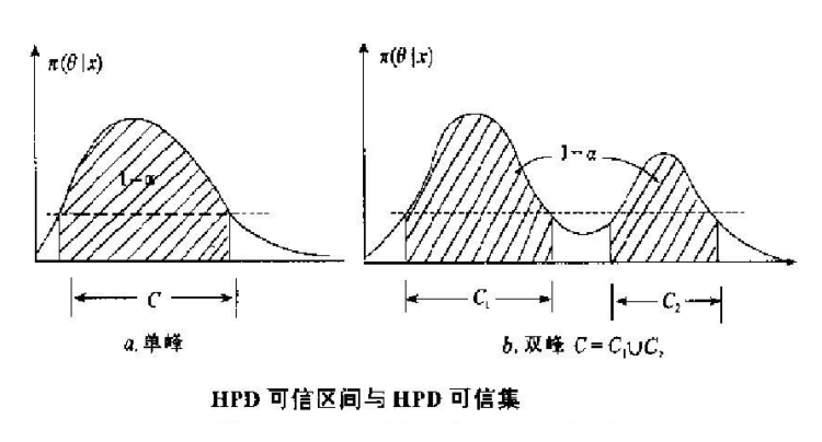
Some explanations.

Some basic explanations for a credible HPD zone

The reprocessing of discrete random variables is difficult to calculate and generally does not study.
A single post-peak density of HPD is always available.
Multi-peak post-density often gives HPD credibility to multiple unconnected zones. Set About multi-peak post-density
The emergence of multi-peak post-density is often caused by inconsistencies between a priori and sample information, which are important for Bayesian statistics.
Co-prospecting is mostly single-peak, which must lead to a single-facing distribution, which may conceal the many-facility resistance that should have been generated, so be careful to use co-prospecting. You should be careful when using a credible HPD.
HPD Trusted Areas are not strictly Trusted Areas
The HPD trust zone is also a symmetrical zone at single peaks;
(b) When single peaks, asymmetrics, solve by computer numerical methods;
When multiple peaks, recommend abandoning HPD guidelines and using a connected symmetrically credible zone estimate

Computer asymmetrical HPD trustable range for the solver of a single-scale value

In fact, the process of the intertinction of computers is very well understood.

Give the initial$k$Value
Calculate$\pi(\theta|x)=k$ Got it.$\theta_1,\theta_2$
Calculate$\theta_1,\theta_2$Go, go, go!$\pi(\theta|x)$%1 points
If the confidence is greater than what is required, increase it.$k$ Otherwise, it's down.$k$ Continue with the iterative phase two. It's enough to understand that.

Large sample method

In the case of large samples, use a near HPD-like trustable zone.

Proof of: $n$ The blogger says:$\pi_n(\theta|x)$Close to obedience. $N(\mu^\pi(x),V^\pi(x))$ Here$\mu^\pi(x)$and$V^\pi(x)$Aftervalid averages and backer averages, respectively Bad

He's a symmetrical single-peak distribution, a consistent HPD-respondent zone and a symmetrical zone. Out$\theta$ The level of credibility is similar to 1-$\alpha$ And the HPD zone is $$(\mu^\pi(x)-u_{\alpha/2}\sqrt{V^\pi(x)},\mu^\pi(x)+u_{\alpha/2}\sqrt{V^\pi(x)})$$

Big samples don't need to calculate the posteriori distribution. Take a rather interesting example of a large sample of HPD. Number of weekly fire incidents in a currency X Subject to Porpine distribution $P(\theta)$, no information a priori distribution of the thorium is known, and no information a priori is considered$\pi(\theta)=\theta^{-1}I_{(0,\infty)}(\theta)$ is appropriate. Set the total number of fire incidents in 5 weeks to be 3 with a mean distribution of porcelain $\theta$ The level of credibility is 90% of the HPD trustable area, using a large sample method; We should be able to calculate the post-censorship distribution, but five observations in five weeks, and we only have three total observations. The core of the Porcelain distribution is $$\theta^ke^{-\theta}$$ We might want to take a look at 11,100 over the next five weeks. So the sample combines to be $$\theta^3e^{-5\theta}$$ So the back-up distribution is positive. $$\theta^2e^{-5\theta}$$ This is the base of Gamma's distribution, and the average of the posteriori distribution is calculated as $\frac{3}{5}$ Square difference$\frac{3}{25}$ Based on the large sample method, there's a study.$N(\frac{3}{5},\frac{3}{25})$90% HPD, the trustable zone, because the normal distribution is symmetrical, the study can wait for the trustable zone.

Assumptions test

The hypothetical test is also a major category of questions studied throughout classical statistics, and after the estimates are completed, it is natural to test the reasonableness of our estimates, and to test the statistical levels of assumptions in the classical statistics, which are more than the need to construct them;

General hypothetical test method

Assumptions in classic statistics

Create original assumptions$H_0$and alternative assumptions$H_1$
Select the number of tests$T=T(x)$ When the original assumption is$H_0$When it's true, it's known.
Visibility of the given$\alpha$ The probability of making a first-class error is less than the probability of a denial.$\alpha$
Sample observation values$x$When you fall in the rejected domain, you reject the original hypothesis.$H_0$ Otherwise, the original assumption is retained

As with the construction of the pivotal, it is difficult to test the determination of statistics in classical statistics.

Assumptions in Bayes statistics

Probability of post-testing$\pi(\theta|x)$ Then calculate assumptions separately$H_0$ $H_1$ Post-probability $\alpha_i=P(\theta_i|x)$
When the probability ratio is back-checked>1$ 时不拒绝$H_0$ $\frac{\alpha_0}{\alpha_{1}}<1$ 时不拒绝$H_{1}$ 接近$A $1-million period without judgment, without any conclusion.

A comparison of hypothetical thinking between schools

It's easy to see.

The Bayesian hypothesis test is easier to understand, simpler.
The Bayesian hypothetical test does not need to select the statistical test to determine the sample distribution
No prior indication of a significant level of visibility to determine the area of rejection
It's easy to extend to multiple hypotheticals or to look for the highest probability of a posteriori.

In fact, the Beyers statistical hypothetical test is the same as the classic statistical principle of probability, but it doesn't require counter-proofing.

Details of the Bayesian hypothetical test

We're here to tell you how to do the Bayesian hypothetical tests.

Post-probability density calculations: a little Assumptions$H_0$ Assumptions$H_1$ $H=H_{0}\cup H_1$ For the total space, all the assumptions mean$\theta\in H$

Calculation assumptions$H_0$ Post-probability $P(H_0|x)=\int_{H_0}^{}\pi(\theta|x)d\theta\triangleq\alpha_0$
Calculation assumptions$H_1$ Post-probability $P(H_1|x)=\int_{H_1}^{}\pi(\theta|x)d\theta\triangleq\alpha_1$
Calculate the probability ratio for post-test$\frac{\alpha_0}{\alpha_{1}}$

$\frac{\alpha_0}{\alpha_{1}}>1$ 时不拒绝$H_0$ 也就是接受$H_0$
$\frac{\alpha_0}{\alpha_{1}}<1$ 时不拒绝$H_{1}$ 也就是接受$H_1$
$\frac{\alpha_0}{\alpha_{1}}\approx 1$ No judgement, no conclusion, further sampling or a priori correction.

The hypothetical test in Bayes statistics is being translated into a problem of points.

Simple assumption: the assumption we're making at this time is$\theta=x$
Complex assumptions: assuming the corresponding parameters are valued as a space

Beyes Factor and Presumption Test

The Beyers factor can help us understand better the Beyers hypothetical test.

Two assumptions$\Theta_{0}$and$\Theta_{1}$The probabilities are the same.$\pi_0$and$\pi_1$, the probability of a later examination is different$\alpha_0$and$\alpha_1$, and then $$B^\pi(x)=\frac{\text{后验机会比}}{\text{先验机会比}} = \frac { \alpha _ 0 / \alpha _ 1 }{ \pi _ 0 / \pi _ 1 }=\frac{\alpha_0\pi_1}{\alpha_1\pi_0}$$ Bayes factor

I can see that.

The Beyers factor depends on data at the same time.$x$& A priori Distribution$\pi(\theta)$
Two opportunities, compared to dichotomy, reduce the a priori distribution, and highlight the impact of data.
Bates factor reflects data$x$Support the original assumption$H_0$The extent of the system (as with the opportunity to divide by one)

Simple assumptions versus simple assumptions

Now we're looking at the Beyers factor in a few different scenarios, and we're continuing to strengthen the most central hypothesis test we've given: the probability ratio.

First, look at simple assumptions. Assumptions are: $$H_{0}:\Theta_{0}={\theta_{0}}\leftrightarrow H_{1}:\Theta_{1}={\theta_{1}}.$$ There's a chance of a corresponding post-test. $ \begin{aligned}\alpha 0&=P(\Theta_0|\boldsymbol{x})=\frac{f(\boldsymbol{x}|\theta_0)\pi_0}{f(x|\theta_0)\pi_0+f(\boldsymbol{x}|\theta_1)\pi_1},\\alpha_1&=P(\Theta_1|\boldsymbol{x})=\frac{f(\boldsymbol{x}|\theta_1)\pi_1}{f(\boldsymbol{x}|\theta_0)\pi_0+f(\boldsymbol{x}|\theta_1)\pi_1},\end{aligned}$$ It's a definition of the probability, and it's easy to calculate because it corresponds to the discrete probability space.

So, the chance is the one. $$\frac{\alpha_0}{\alpha_1}=\frac{\pi_0f(\boldsymbol{x}|\theta_0)}{\pi_1f(\boldsymbol{x}|\theta_1)}$$ Calculating the Beyers Factor $$B^\pi(\boldsymbol{x})=\frac{\alpha_0/\alpha_1}{\pi_0/\pi_1}=\frac{f(\boldsymbol{x}|\theta_0)}{f(\boldsymbol{x}|\theta_1)}.$$ You want to reject the original hypothesis, which is to ask for $\frac{\alpha 0}<1$ 也就是$$\frac{f(\boldsymbol{x}|\theta_1)}{f(\boldsymbol{x}|\theta_0)}>\frac{\pi_0}{\pi_1}.$$

Intuitive understanding is that the density function is more than the threshold, which is similar to the basic result of N-P reasoning.

From now on, it's obvious. $B^\pi(\boldsymbol{x})$ It's supposed to be a ratio of opportunity to data, and he's not dependent on a priori distribution, but on the sample.
So we're taking the Beyers.$B^\pi(\boldsymbol{x})$ Consider Data$x$- Yes.$H_0$Level of support

Complex assumptions versus complex assumptions

Calculating the Beyers Factor

Considering the following hypothetical test issues: $$H_0:\theta\in\Theta_0\leftrightarrow H_1:\theta\in\Theta_1,$$ And we can re-write the a priori density function in the following form.The rewriting is intended to facilitate the subsequent calculation and representation. $$\left.\pi(\theta)=\left{\begin{array}{ll}\pi_0g_0(\theta),&\theta\in\Theta_0,\\pi_1g_1(\theta),&\theta\in\Theta_1,\end{array}\right.\right.$$

Rewrite the probability ratio under this mark. $$\frac{\alpha_0}{\alpha_1}=\frac{\int_{\Theta_0}f(\boldsymbol{x}|\theta)\pi_0g_0(\theta)\mathrm{d}\theta}{\int_{\Theta_1}f(\boldsymbol{x}|\theta)\pi_1g_1(\theta)\mathrm{d}\theta},$$ The form of the fraction is that complex density functions do not need to process single points. Give me the Bates. $$B^\pi(\boldsymbol{x})=\frac{\alpha_0/\alpha_1}{\pi_0/\pi_1}=\frac{\int_{\Theta_0}f(\boldsymbol{x}|\theta)g_0(\theta)\mathrm{d}\theta}{\int_{\Theta_1}f(\boldsymbol{x}|\theta)g_1(\theta)\mathrm{d}\theta}=\frac{m_0(\boldsymbol{x})}{m_1(\boldsymbol{x})}.$$ The ratio of the border-distribution.

Explain the Beyers.

The Beyers factor at this time is not an apparent comparison, but it can be seen as an apparent weighting form, partially eliminating the effects of the a priori distribution, emphasizing the sample.
If you set up a new one,0$ 与$\hat{\theta}1$ 分别是$\theta$在$\Theta{0}$与$\Theta{1}$上的极大似然估计(MLE), 那么经典统计中所使用的似然比统计量是贝叶斯因子$Special case of $ ^ (\mathbf{x}
The response of the Beyers factor to changes in sample information is sensitive, while the reaction to changes in a priori information is slow (this is explained by the complexity and complexity of the information, and simply by the fact that the Beyers factor and the a priori are completely irrelevant to the simple assumption)

Simple assumptions versus complex assumptions

Considering the following hypothetical test issues: $US$US$US$US$US$US$US$US$US$US$US$US$US$US$US$$US$US$US$US$US$US$US$US$$US$$US$US$US$US$$US$US$US$$US$$US$$US$US$US$$US$US$US$US$$US$$US$US$$US$$US$$US$$US$$$$$US$$$US$$$US$$$$US$$$$$$$$$$$$$$$$$$$$$$$$$$$$$$$$$$$$$$$$...$$$$$$$$$...$$$$$...$$$$$$$$$...$$$$$...0：\theta=\theta1 \theta\neq\theta $0 This is the most complicated situation.

If we use a continuous density function directly, then the a priori probability of a single point must be zero, and there's no way to calculate it. So we need to solve the problem by rewriting the density function in a complex and complex way to add parameters.

- There's a deformation. $$\pi(\theta)=\pi_0I_{\theta_0}(\theta)+\pi_1g_1(\theta)$$ Of which$I$It's a token function that's added to it.$\theta=\theta_0$. Time to take to 1 $\pi_0+\pi_1=1$ We can assume that the a priori density at this time is composed of two separate and continuous parts, so there is a certain number of people who are separated from each other. $$\left.\pi(\theta)=\left{begin{array}ll}pi 0,&\theta=\theta_0,\\pi_1g_1(\theta),&\theta\neq\theta_0,\end{array}\right.\right.$$ 计算边缘密度有 $$m(\boldsymbol{x})=\int_\Theta f(\boldsymbol{x}|\theta)\pi(\theta)\mathrm{d}\theta=\pi_0f(\boldsymbol{x}|\theta_0)+\pi_1m_1(\boldsymbol{x}),$$ 其中$m_1(x)$为$$m_1(\boldsymbol{x})=\int_{\theta\neq\theta_0}f(\boldsymbol{x}|\theta)g_1(\theta)\mathrm{d}\theta.$$ 分别计算两个假设下的后验密度有 $$\alpha_0=\pi(\Theta_0|\boldsymbol{x})=\frac{\pi_0f(\boldsymbol{x}|\theta_0)}{m(\boldsymbol{x})},\quad\alpha_1=\pi(\Theta_1|\boldsymbol{x})=\frac{\pi_1m_1(\boldsymbol{x})}{m(\boldsymbol{x})}.$$ 因此可以计算后验机会比 $$\frac{\alpha_0}{\alpha_1}=\frac{\pi_0f(\boldsymbol{x}|\theta_0)}{\pi_1m_1(\boldsymbol{x})}.$$ 计算贝叶斯因子有 $$B^\pi(\boldsymbol{x})=\frac{\alpha_0/\alpha_1}{\pi_0/\pi_1}=\frac{f(\boldsymbol{x}|\theta_0)}{m_1(\boldsymbol{x})}.$$

It is easier to see the Beyers factor in its presentation, and there are no parameters that we have added to the study to support it, so we tend to calculate the Beyers factor in the actual study, and using the Beyers factor to calculate the probability later is a simple equation.

One example

This example is not about the knowledge of computation. We have to explain the results of the calculations.

Set From Normal General$\mathbb{N}(0,1)$randomly extract a capacity as$10$The sample x, the average sample value $\overline{x}=1.5$, test two assumptions: I'm sorry. H 0: \theta\leq 1, \quadH 1:\theta>1 $$ $\text{取}\theta\text{的共轭先验分布为N}(0.5,2)\text{}$

Obviously complex, complex, and the chances of a later check on formula calculations. - Yeah. $ \begin{aligned}\alpha 0=&\mathrm{P(\theta\leq1|x)=0.0708}\\alpha_1=&\mathrm{P(\theta>1|lpha 0=0/922}end{aligned}$$$ Post-opportunity versus support assumptions$H_1$

Calculate a priori chances against $$\pi=0.6368,\quad\pi_1–0.3632$$ A priori opportunity against support$H_0$

Calculating the Beyers. $$B^\pi(x)=0.0434$$ The Beyers factor supports the hypothesis.$H_1$

It's a contradiction between our beyers and our a priori judgment, and it's a response to our conclusions. The Beyers factor is more concerned with sample information, and in fact this phrase is valid for any type of beyers hypothetical test.

Projections extrapolation

We're making statistical inferences about the future observations of random variables, and there's no chapter in mathematical statistics that corresponds to them.

A brief introduction.

What we need to do is estimate the future observations of random variables based on the situation that is known, which will basically be divided into the following:

No observations, parameters$θ$Unknown, forecast$X$（$X$Organisation$\theta$(parameters)
Observation information, parameters$θ$Unknown, forecast$X$（$X$Organisation$\theta$(parameters)
Observation information, parameters$θ$Unknown, forecast$Z$（$Z$Organisation$\theta$(parameters)

Projections in the absence of observations

And although we don't have any observations at this point, there's a sample distribution and a priori distribution of parameters, which naturally gives a marginal distribution. $$m(x)=\int_{\Theta}p(x|\theta)\pi(\theta)d\theta $$ As our forecast distribution, this is called a priori projection distribution.

Projections methods: Use the projection of the expected, median or agglomerations of the projected distribution (as we did in the Bayesian point estimate)

Use a certain confidence to calculate the confidence interval for the projected distribution (as we did in the Bayesian estimation)

If you have X-observation data, predict X.

Calculates post-femination$\pi(\theta|{x})$ We calculate our projected distribution using a posteriori density. $$m(x\mid\mathbf{x})=\int_{\Theta}p(x\mid\theta)\pi(\theta\mid\mathbf{x})d\theta $$ Called the Post-Examining Forecast Distribution The projection methodology remains unchanged

When X observations are available, predict Z.

Calculates post-femination$\pi(\theta|{x})$ We calculate our projected distribution using a posteriori density. $$m(z\mid\mathbf{x})=\int_{\Theta}g(z\mid\theta)\pi(\theta\mid\mathbf{x})d\theta $$Called the Post-Examining Forecast Distribution The projection methodology remains unchanged

Bates Hypothesis and Model Selection

Multi-scenario Bayesian hypothetical test

The previous hypothetical test is limited to the link between the original and alternative assumptions Bayesian Statistics 1 (Beyes Statistics and Post-Assessment Distribution) The Beyes Hypothetical Test and Model Choice section, however, an important advantage of the Beyes Hypothetical Test is that it is very easy to extend to multiple scenarios;

We just need to calculate the back-probability ratio or the Beyers factor between the multiple assumptions, and we can only decide whether we accept the original assumption according to its size;

And as for the size of the Beyers factor, the relationship to the assumptions on the model support molecule, Jeffeys made some suggestions.

Bayesian	Interpretation
$B<1$	Negative molecular assumptions
$1<B<3$	Insufficient evidence of hypothetical evidence on the supporting molecule
$3<B<10$	Strong support
$10<B<30$	Strong support.
$30<B<100$	Very strong support.
$100<B$	I'm sure you'll support it.

Assessment of the Bayesian model

Importance of the Bayesian model evaluation

Both the Beyers statistical extrapolation and decision-making are dependent on the later distribution; therefore the results of the extrapolation study are dependent on the quality of the later distribution; it is therefore important to evaluate our Beyers model; the usual Bayes model evaluation method includes not only the AIC BIC guidelines introduced from classical statistics, but also the BPIC.

AIC and BIC

They're all based on the principle of great apparition, the MLE estimate.Mathematical statistics The "Big Appearances" section. Build

The AIC Guidelines are in the form of $AIC=2\f\lft(x)\widinghat(theta)}+2p, $ Where's the \\wideehat(theta)?{MLE}is the largest estimate of \theta \left (MLE\right)$ $P$ is the dimension of the estimation parameter

The BIC guidelines take the form of: $$BIC=-2\ln f\left(x_{n}|\widehat{\theta}_{MLE}\right)+p\ln n$$ We're both aiming to be small.

BPIC BPIC BEC BEC BEC BIENZ BEYES

Consider the following two assumptions: (a) Parameter model $f(x|\theta)$ It contains a real model. $g(x)=f(x;\theta_0)$ $\theta_0\in\Theta$, and the specified model is not far from the real model; (b) the logarithmic a priori is $\ln\pi(\theta)=O_p(1).$ Ando (2007) presents the Bayesian forecast information guidelines (the Bayesian forecast profile, BPIC) under the two above-mentioned assumptions and certain normal conditions. $$ BPIC=-2\int_{\Theta}\ln f\left(x_{n}|\theta\right)\pi\left(\theta|x_{n}\right)d\theta+2p, $$

Because the logarithmic posterior averages are not usually analyzed, we usually approach the MC method. $$\int_{\Theta}\ln f\left(x_{n}|\theta\right)\pi\left(\theta|x_{n}\right)d\theta\approx\frac{1}{L}\sum_{j=1}^{L}\ln f\left(x_{n}|\theta^{\left(j\right)}\right),$$ This is a less a priori.

DIC Code for Distortion Information

You!$D\left(\theta\right)=-2\ln f\left(x_{n}|\theta\right)$It's a measure of the usual model deviation. Spiegelhalter et al. (2002) points to a similar backsight. $\bar{D}=E[D(\theta)|x_n]$The higher the model's data is, the higher the model's data is, the higher the model's data is, the higher the model's data is, the more the model's data is, the more the model's data is, the more the model is, the more the data is, the more the data is, the more the data is, the more the data is, the more the data is, the more the data is, the more the data is, the more the data is, the more the data is, the more the data is, the more the data is, the more the data is, the more the data is, the more the data is, the more the data is, the more the data is, the more the data is, the more the data is, the more the data is, the more the data is, the more the data is, the more the data is, the more the data are, the more the data are, the more the data are, the more the data are the data are the data are the data, the more the data are the data are the more the data are the data are the data that are the data are the data are the data.$\bar{D}$ The smaller the number of valid parameters is defined below to characterize the complexity of the model: I'm sorry. P D=overline{D}-D(overline{theta}{n})=2\ln f(\boldsymbol{x}{n}|\overline{\boldsymbol{\theta}}{n})-2\int{\Theta}\ln f(\boldsymbol{x}{n}|\boldsymbol{\theta})\pi(\boldsymbol{\theta}|\boldsymbol{x}{n})\mathrm{d}\boldsymbol{\theta}, $$

of which$\vec{\theta}_n$ Defines the deviation information guidelines for the later average. Spiegelhalter et al. (2002) (Deviance Information profile, DIC) as

$$ DIC=\overline{D}+p_{D}=-2\int_{\Theta}\ln f\left(x_{n}|\theta\right)\pi\left(\theta|x_{n}\right)\mathrm{d}\theta+p_{D},\left(4.6.13\right) $$ The first one. $\tilde{D}$ It can be explained as a measure of the degree of model alignment, the smaller the better; second $p_D$ Considered a measure of the complexity of the model, as defined above $DIC$ Could be rewritten to $DIC=D\left(overline {\theta}{n}\right)+$ $2p{D}=-2\ln f\left(\boldsymbol{x}{n}|\overline{\boldsymbol{\theta}}{n}\right)+2p_{D}$,其中$\overline{\boldsymbol{\theta}}{n}$ 为后验均值，从形式上看，它与 AIC 很相似，因此可以认为 $DIC$ 是 $AIC=D(\widehat{\theta}{MLE})+2p$ 的一个推广，此处 $\widehat{\theta}{MLE}$ 为$\theta$ 的最大似然估计，对非分层模型而言，当$n$ 充分大时有 $p\approx p_D,\widehat{\theta}♪ And I'm gonna be a big fan of the world ♪

DEC can easily calculate the results by using the MCMC method. So the DIC guidelines are used for a variety of beyers model selection problems.

Statistical decision-making

Introduction

In addition to the three elements of statistical decision-making: sample space and distributed family space loss function, the Beyers statistical decision-making introduced the fourth element of pre-spect distribution function based on statistical decision-making.$F(\theta)$

The Beyers statistical decision-making introduced a fourth element based on the Beyers statistical extrapolation.$L$

Here we make a deal: If data for decision-making are not randomly influenced, it is called a general decision-making issue (all defined decisions fall into this category). On the contrary, if you get random effects, it's called statistical decision-making.

Minimum principle of post-risk

The principle of the lowest risk is as important for statistical decision-making as the probability of post-mortem is for statistical inference.

Definition of post-examining risk

We call the loss function a posteriori risk function. $$R(\delta(x)|x)=E^{\boldsymbol{\theta}|x}[L(\theta,\delta(x))]$$ $$\left.=\left{\begin{array}{l}\int_\Theta L(\theta,\delta(x))\pi(\theta|x)\mathrm{d}\theta,\\sum_iL(\theta_i,\delta(x))\pi(\theta_i|x),\end{array}\right.\right.$$ He and Bayes expected to lose in the same vein, a probabilities using a priori and a probabilities using a posteriori.

If the decision function is to minimize the risk of post-risk, we call it the best Beyers decision-making function under the Minimal Risk Standard.

Relationship between post-risk and Bayesian risk

We know that in the Bayesian statistical inferences. $$f(x,\theta)=f(x|\theta)\pi(\theta)=\pi(\theta|x)m(x)$$ This is the late distribution formula migration.

Use it to transform the Beyers risk. $$R_{\pi}(\delta(x))=E^{\theta}\bigl[R(\theta,\delta(x))\bigr]=E^{X}\bigl[R(\delta(x)|x)\bigr]$$ The core of the Beyers solution, which is used to calculate the Beyers solution, is expressed in two equals. Pattern

One is to calculate the risk function and then use a priori probability density.$\pi(\theta)$Average The other one is to calculate the risk and then use the edge distribution.$m(x)$Average

It proves that $$00\ R (\delta)& =E^{\theta}[R(\theta,\delta(x))] \ &=\int_{\Theta}R(\theta,\delta(x))\pi(\theta)d\theta \ &=\int_{\Theta}\int_{\chi}L(\theta,\delta(x))f(x\mid\theta)\pi(\theta)dxd\theta \ &=\int_{\chi}\biggl[\int_{\Theta}L(\theta,\delta(x))\pi(\theta\mid x)d\theta\biggr]m(x)d\mathbf{x} \ &=E^{\mathrm{x}}\Big[R(\delta(x)|x)\Big], \end{aligned}$$

Minimum principle of post-risk

We will prove:The decision-making function under the principle of minimal risk is Bayes. Break Theorem: There exists a non-random decision-making function $\delta_{\pi}(x)$,Fulfilment of Conditions I'm sorry. R (\) =pectorname* *inf*{\delta}R(\delta(x)|x)=\operatorname*{inf}I'm not a real guy. I'm sorry. then $\delta_\pi(x)$ A priori distribution $\pi(\theta)$ The Bhaius solution. $\pi(\mathrm{d}\theta|x)=\pi(\theta|x)\mathrm{d}\theta.$

If$\pi(\theta)$We've got a broad beyers solution, but the a priori formula doesn't change. We understand the complexity of the concept.

Proofs that: $$\begin{aligned}R(\delta(x)|)&=\int_\Theta L(\theta,\delta(x))\pi(\mathrm{d}\theta|x)\&\geqslant\int_\Theta L(\theta,\delta_\pi)\pi(\mathrm{d}\theta|x)=R(\delta_\pi(x)|x),\end{aligned}$$ 两边同时对边缘分布$m(x)$做积分有 $$\begin{aligned} R_{\pi}(\delta(x))& =\int_{\mathcal{X}}R(\delta(x)\mid x)m(x)\mathrm{d}x \ &\geqslant\int {\mmathcal{x)m(x)\mathrm{d}x=R\pi(\delta \pi(x)). I'm sorry, I'm sorry. It proves that the lowest risk of post-examining is Bayesian, the least risk of the post-examining is Bayesian. Break

A simple example.

Set$\theta$The a priori distribution is $\pi(\theta_1)=0.6~\pi(\theta_2)=0.4$ Set Random Variables$X$Take 0-1 2 values$p(i|\theta_j)=P(X=i|\theta=\theta_j)$ Yes.$X$is the probability distribution $$p(1|\theta_1)=0.1,\quad p(1|\theta_2)=0.2,\quad p(0|\theta_1)=0.9,\quad p(0|\theta_2)=0.8.$$ Calculating the probability of a posteriori if we know the loss function is$L$ Calculating Post-Aspect Risk

The post-exposure of discretes is always more round, not as much as a continuum, but essentially a formula for calculation. $$\pi(\theta_i|x)=\frac{f(x|\theta_i)\pi(\theta_i)}{\sum_if(x|\theta_i)\pi(\theta_i)}\quad(i=1,2,\cdots).$$ According to the theory, we're going to calculate the probability of a back check in two samples.$X=0$ And the other one is...$X=1$ When we calculate the edge density, don't replace it with specifics.$\theta$, 'cause I'm gonna take all of it

The risk of post-loss is the loss function's after-feed density points, both in profit and loss matrix and in continuous functions.

Bates estimate under the general loss function

We use the decision-making method to consider the question of the beyers point estimates in statistical extrapolation.

And the last beyers that you get is the estimate of the parameters that you want to be asked for in the question.

Bayesian estimate under the square loss function

If the loss function is used $$L(\theta,\delta)=(\delta-\theta)^{2}$$ Then we know.$\theta$The Bates estimate is the posteriori average, which is $$$$$$$$$$$$$$$$$$$$$$$$$$$$$$$$$$$$$$$$$$$$$$$$$$$$$$$$$$$$$$$$$$$$$$$$$$$$$$$$$$$$$$$$$$$$$$$$$$$$$$$$$$$$$$$$$$$$$$$$$$$$$$$$$$$$$$$$$$$$$$$$$$$$$$$$$$$$$$......$$$$$$$$$$$$$......$$$$$$$$...$$$$$$$$$...$$$...$$......$$$.........$$$$$$$$$$$$$$$...........................$$$$$$$$$$$$$$$$$$$$$$$$B}(x)=E(\theta|x)$$ 证明如下： $$\begin{gathered} R(a|\boldsymbol{x}) =E[(\theta-a)^2|x]=\int\Theta(\theta-a)^2\pi(\theta|\boldsymbol{x})\mathrm{d}\theta \ =\int_{\Theta}(\theta^{2}-2a\theta+a^{2})\pi(\theta|\boldsymbol{x})\mathrm{d}\theta. \end{gathered}$$ 我们需要找到合适的$a$ 让后验风险最小对$a$求偏导有 $$\mathrm{\mathrmbl}{\d}theta+2a=$0.00= And so...$a$ Minimise when equal to the posteriori average

Right there.$\Theta$The upper-to-prevalence density function, the after-test density function is all one, which is determined by the nature of the density function.

Form of the weighted square loss function If the loss function is used $$L(\theta,\delta)=w(\theta)(\delta-\theta)^{2}$$ Then we know.$\theta$The Bayesian is probably... $$$$$$$$$$$$$$$$$$$$$$$$$$$$$$$$$$$$$$$$$$$$$$$$$$$$$$$$$$$$$$$$$$$$$$$$$$$$$$$$$$$$$$$$$$$$$$$$$$$$$$$$$$$$$$$$$$$$$$$$$$$$$$$$$$$$$$$$$$$$$$$$$$$$$$$$$$$$$$......$$$$$$$$$$$$$......$$$$$$$$...$$$$$$$$$...$$$...$$......$$$.........$$$$$$$$$$$$$$$...........................$$$$$$$$$$$$$$$$$$$$$$$$B}(x)=\frac{E[w(\theta)\theta|x]}{E[w(\theta)|x]}$$ 他的计算式为也就是对后验密度求期望 $$\frac{\int_a\theta w(\theta)\pi(\theta\mid x)\mathrm{d}\theta}{\int_aw(\theta)\pi(\theta\mid x)\mathrm{d}\theta}$$ 这个期望的计算还是比较复杂的一般是构造新的分布积分为1实现证明如下 $$\begin{aligned} R(a|\boldsymbol{x})& =E\bigl[w(\theta)(\theta-a)^2|\boldsymbol{x}\bigr] \ &=\int{\boldsymbol{\Theta}}\left[\theta^2w(\theta)-2a\theta w(\theta)+a^2w(\theta)\right]\pi(\theta|\boldsymbol{x})\mathrm{d}\theta. \end{aligned}$$ 求偏导有 $$\mathrm{\mathrm{d}a}ta\bardsymbol=)=mathrm=d} The equation will lead to the conclusion.

When the parameter vector is multiple $\theta^{\prime}=(\theta_1,\cdotp\cdotp\cdotp,\theta_k)$ For Multiple Diplesity Loss Functions $$L(\theta,\delta)=(\delta-\theta)^{\prime}Q(\delta-\theta)$$ Bates estimates the post-mortem average. $$\delta_B(x)=E(\theta\mid x)=\begin{pmatrix}E(\theta_1\mid x)\\vdots\E(\theta_k\mid x)\end{pmatrix}$$

Bates estimate under the linear loss function

We take the loss function as linear. $$L(\theta,\delta)=\begin{cases}k 0(theta-\delta),\delta\leq\theta\k 1 (\delta-\theta),\delta>\theta&You're not gonna get away with this? His Bayes is probably a posteriori distribution.$\pi(\theta|x)$ Yes.$\frac{k_0}{k_{0}+k_{1}}$Bits

Special if the loss function is (i.e., the absolute value loss function) $${L}(\theta,\delta)=|\theta\text{-}\delta|$$ Bates is estimated to be a posteriori median.

Practicability and limited operational issues

In estimating the problem, action is often a matter of choice, but many statistical decision-making issues are only available in a limited number of actions, such as hypothetical testing, and the question of the Bayesian statistical decision-making is very well handled.

Space of operation $A={a_{1},a_{2},...,a_{r}},$ Losses are as at $L(\theta,a_i)$ To find the best, we have to get back to the expected loss. $E^{\theta|\mathbf{x}}[L(\theta,a_i)]$ Minimum

Two issues are examined below: two actions (assuming tests) multi-action (classification) issues

Presumption test issues

Consider the following hypothetical test issues: $$H_0:\theta\in\Theta_0\leftrightarrow H_1:\theta\in\Theta_1\quad(\Theta_0\cup\Theta_1=\Theta).$$ Use action$a_0$- To accept the original assumption. - Action.$a_1$ To deny the original assumption

Select$0-k_i$The loss function is as follows: $$\left.L (\theta,a 0)=\left(begin{array}ll}0,&\theta\in\Theta_0,\k_0,&\theta\in\Theta_1,\end{array}\right.\right.$$ $$\left.L(\theta,a_1)=\left{\begin{array}{ll}k_1,&\theta\in\Theta_0,\0,&\theta\allay.\right.\right.$ It's a function of operational space and parameter space, of course.

Post-risk $$\begin{gathered} R(a_0\mid x)=E^{\theta\mid x}[L(a_0,\theta)]=\int_{\Theta_1}k_0\pi(\theta\mid x)d\theta=k_0P(\Theta_1\mid x) \ R(a_1\mid x)=E^{\theta\mid x}[L(a_1,\theta)]=\int_{\Theta_0}k_1\pi(\theta\mid x)d\theta=k_1P(\Theta_0\mid x) \end{gathered}$$ You can just use the back-up risk criterion to determine the best course of action when comparing the size of the back-up risk.

There's a presumption against it. $$k_0P\left(\Theta_1|x\right)\geqslant k_1P\left(\Theta_0|x\right),$$ Equivalent $$P\left(\Theta_{1}|x\right)\geqslant\frac{k_{1}}{k_{0}+k_{1}}.$$ This is the rejection of the Beyers hypothetical test in the classic statistics. $$D=\left{X=\left(X_{1},X_{2},\cdots,X_{n}\right):P\left(\Theta_{1}|X=x\right)\geqslant\frac{k_{1}}{k_{0}+k_{1}}\right},$$ We've seen this form in the seemingly comparable test.

Multi-action issues

The way we deal with the problem of multiple operations has not changed, and for each operation we give the expression of the loss function independently.

The loss function is based on a relatively reasonable choice.

And then we calculate the risk of post-examining, and compare the size of the post-examining risk to make the final decision, the same idea as we did when we studied the hypothesis test directly in front. Bayesian Statistics 1 (Beyes Statistics and Post-Assessment Distribution) and the “Beyers Presumption and Model Selection” section

Inter-district estimates in statistical policymaking

Consider applying statistical decision-making methods to consider the issue of credible inter-temporal or inter-temporalization

At this point, the operational space is the assembly of all possible inter-zone formations.$C(x)=[d_{1}(x),d_{2}(x)]$ Loss function is used to $$L(\theta,C(x))=m_1[d_2(x)-d_1(x)]+m_2[1-I_{C(x)}(\theta)]$$ Of which$m_1~m_2$It's a constant given in advance. The first half measures the loss from the length of the zone, the greater the loss. The second half of the story is that$\theta$Losses from deviations

Compare the risk of post-examining between multiple zones, and find the least risk of post-examining.

Minimax Guidelines

Consistent optimal decision-making functions may not exist, or often do not; then we need a new guideline that considers which best from the point of view of risk functions. This is what we do when we're not sure about a priori distribution. In other cases, it's better to study the later risk.

Consider risk functions$R(\theta,\delta)$ Bayesian Statistics 1 (Beyes Statistics and Post-Assessment Distribution) ..the "Risk Functions and Consistency Best Decision-Making Functions" section $$M(\delta)=\sup_{\theta\in\Theta}R(\theta,\delta).$$ And we look at the most risks in a decision-making situation, and we choose the least risk-taking decision-making. This decision-making rule we call...Minimax Guidelines

The Minimax Code is a mind that doesn't demand much, but that doesn't want much to be lost.

It's more difficult to calculate the Minimax solution. Set $\widiehat{g} k=\widiehat{g}k(\boldsymbol{x})$ 为在先验分布 $\pi_k(\theta)$ 下 $g(\theta)$ 的一列贝叶斯估计，$k=1,2,\cdots;$ 假定 $\widehat{g}k$ 的贝叶斯风险为 $r_k,k=1,2,\cdots$, 且有$\lim{k\to\infty}r{k}=r<\infty$,
Set $\widiehat{g}}=\widehat{g}^{}(x)$ 为 $g (\theta) $$1 = an estimate, condition fulfilled $M\left (\wideehat{g}{\cHFFE7C5}right, {\cHFFE7C5} ^Minimax estimates for decision-making

Bayesian statistical calculations

Introduction

(a) The expectations, differences, fractions or numbers of post-square distributions are often calculated in the Bayesian statistical methodology; For example, the usual post-mortem average, which is estimated by Beyers at the square loss, is measured by the difference between the post-test examination ... the post-censorship number, the post-test median and the post-test fractional number are also often used as a factor in the Yates estimation or in the establishment of a Beneath trustable zone; If the a priori distribution is not its a priori distribution (which is often encountered in many cases), then the later distribution is often no longer a standard distribution. Thus, the numerical characteristics of the posteriori distribution that need to be calculated are often not expressed in a dominant way, which requires some special methods of calculation.

Like what? $$\pi(\theta|x)\propto\exp{-(\theta-x)^{2}/(2\sigma^{2})}[\tau^{2}+(\theta-\mu)^{2}]^{-1}.$$ His posteriori expectations and differences are complex, undissolved points. We can also solve it with some numerical weights.

Think about another question. Aforecast distribution given with logarithmic distribution $$\nu=\left(\ln\theta_{1},\ln\theta_{2},\cdots,\ln\theta_{k}\right)^{T}\sim N\left(\mu1_{k},\tau^{2}\left{\left(1-\rho\right)I_{k}+\rho J_{k}\right}\right)$$ So you can give the later distribution to $$00\&\pi\left(\nu|x\right)\propto f\left(x|\nu\right)\pi\left(\nu\right)\propto g\left(\nu|x\right)\&=xp\left{-\sum l\l\left}}l}l}l}l}l}l l l l mu l\l^l^l\l^l^l\l}l}l}l}l}l}l}l}l}l}l}l}l}l}l}l}l}l}l}l}l}l}l}l}l}l}l}l}l}l}l}l}l\l\l}l\l\l\l\l\l}l}l}l}l}l}l}l}l}l}l}l}l}l}l\l\l}l}l}l}l}l}l}l}l}l\l\l}l}l}l}l}l}l}l}l}l}l}l}l}l}l}l}l}l}lignlignlignlignlignlignlignlignlignlignlignlignlignlignl I'm sorry. His expectations are two.$k$The value of the re-scoring; the value-scoring method is not helping the high-dimensional sub-coordinate (as it relates to the high-dimensional disaster) and now we need some new treatment techniques to solve this problem; of which MCMC algorithms are the most central instrument.

Em algorithm

The EM algorithm is a very important kind of statistical algorithm that he uses to solve two very important statistical computational problems, one of which is a very similar estimation, and the other of the late-calculations in Bayes statistics, which is in fact a special case of the latter, and we focus on the EM algorithm from the perspective of Bayes statistics. EEM algorithms are an extended algorithm (data addition algorithm) because it is very difficult to calculate (extensive) the number of late-calculations directly, but rather to expand some of the original data by adding some potential data, so that a series of large or simulated can be simply achieved. These potential data may be missing data or unknown parameters

The estimate of the post-mortem number is the main use of our EEM algorithm.

Algorithm Process

We're still going to be able to get a later analysis of the distribution.$p(\theta|Y)$ We'll expand into a variable.$Z$ Getting easy${p(\theta|Z,Y)}$ So we can simplify the computation process and then we can add it to the list.$Z$And then we'll make it work.

Em algorithm is an iterative algorithm divided into E step and M step.$p(\theta|Y)$ The post-censorship distribution that means that needs to be studied $p(\theta|Z,Y)$To Add Post-Examining Distribution$p(Z|\theta,Y)$ To expand the condition density function of the variable, our goal is to study the number of numbers that are distributed after the results. Remember$\theta^{i}$It's the first.$i+1$And the next step in the iterative process is to get to the bottom of the count. Step E: Expectation. Yeah.${p(\theta|Z,Y)}$ Or...$log({p(\theta|Z,Y)})$ About$Z$The conditions are based on expectations.$Z$ I'm gonna score it. $$00\ Q (\theta|theta^(i), Y)& \hat{=}E_{Z}\big[\log p(\theta|Z,Y)|\theta^{(i)},Y\big] \ &=\int\big[\log p(\theta|Y,Z)\big]p(Z|\theta^{(i)},Y)dZ. \end{aligned}$$ Here's the expectation of an expanded variable, and we're using an estimate of the number of parameters that are being iterative. Step M, it's huge. - Put it on.$Q(\theta|\theta^{(i)},Y)$ Make it great. Get some.$\theta^{i+1}$ Make $$Q(\theta^{(i+1)}|\theta^{(i)},Y)=\max Q(\theta|\theta^{(i)},Y).$$ Repeat this EEM process until we've been in it.$\theta$Sequence collapse It's huge. By looking for the right thing.$\theta$ Achieved$Q$♪ The great

Theoretically,

Theoretically: If$f(x)$It's a cam function.$$E[f(X)]\leq f[E(X)]$$ It's called Jensen's Instinct.

Theoretically: EEM algorithms can increase the value of a post-density function at every inch. $${p(\theta^{(i+1)}|Y)\geq p(\theta^{(i)}|Y)}$$ Theoretically: If Em's algorithm is in the middle of$\theta$Sequence Satisfaction

$\left.\frac{\partial Q(\theta|\theta^{(i)},Y)}{\partial\theta}\right|_{\theta=\theta^{(i+1)}}=0;$
$\text{d}p(Z\theta^(i), Y\text{softly smooth,}\theta^(i)}\text{deep to certain values}\theta^()♪ I'm not gonna let you go ♪ then $$\partial\log p(\theta|)=$0.00 The EM algorithm must have constricted to a level of stability, but it may not be a maximum value point, but if you want to keep the maximum, you need to select multiple starting values to model stability over time.

Example of an EM algorithm

The missing data is a very significant estimate.

For the general$X\sim N(\mu,\sigma^{2})$ $X_{1},X_{2},X_{3}$ It's a sample from the whole population. $X_{2}$Missing Parameters for determining the overall distribution using a very similar estimate For this type of problem, EEM algorithms can be handled by adding missing data.

Extension$X_{2}$ Get full and symmetrical functions $$\log p(\theta\mid X_1,X_2,X_3)=-3\ln\sigma-\frac{\sum_{i=1}^3(X_i-\mu)^2}{2\sigma^2}.$$ Execute E step, which is directed at$X_{2}$ Expectations. It's obvious.$X_{2}$I'm not expecting anything.$X_{2}$ All of them can be considered constants, so we actually just need to calculate a small fraction. $$E_{X_{2}}[(X_{2}-\mu)^{2}\mid\theta^{(i)},X_{1},X_{3}]=(\mu_{i}-\mu)^{2}+\sigma_{i}^{2}$$ Yeah.$X_{2}$We have the last time we've given an iterative estimate of the parameters. Value$\theta^i$ It's so easy to know.$X_{2}$And finally, what we're looking for is the square of the normal distribution, which is a second-order problem, which is easy to calculate. Then we can get the final results of step E. $$00\ Q (\theta\mid\theta^, X (), X (3),& \left.\hat{=}\left.E_{X_{2}}\right[\log p(\theta\mid X_{1},X_{2},X_{3})\mid\theta^{(i)},X_{1},X_{3}\right] \ &=-3\mathrm{~ln}\sigma-\frac{(X_1-\mu)^2+(X_3-\mu)^2+(\mu_i-\mu)^2+\sigma_i^2}{2\sigma^2}. \end{aligned}$$ M步找到合适的$\theta$取值让Q极大我们只需要研究对$\theta$的偏导数 $$\left.\left[\begin{aligned}&\frac{\partial Q}{\partial\mu}=\frac{(X_1-\mu)+(X_3-\mu)+(\mu_i-\mu)}{\sigma^2}=0,\&\frac(X 1-\m2)^2+ (i-\m2)^sigma 3}=end{aligned}\right.\right.$$ The solution will be the next iterative result. Be careful. We're in the middle of a...$\theta^i$In$\theta^{i+1}$of which$\theta^i$It was something that had to be given when you studied E step. The sequences that are quickly reduced by the overlap are the meaning of the EEM algorithm.

Post-research distribution

In fact, it's very much like studying the distribution of the number of people after studying the function of the function, and the large amount of the missing item is about the problem of the later distribution, and the large amount of the missing item is about a special case of the later distribution of the population.

Assuming there are four possible outcomes, the probability of each happening is that the two of us will be able to do the same. $\frac{1}{2}+\frac{\theta}{4},\frac{1}{4}(1-\theta),\frac14(1-\theta),\frac\theta4,$ of which$\theta$Yes.$(0,1)$The results of the four results were measured as follows:$Y=(y_{1},y_{2},y_{3},y_{4})=(125,18,20,34).$

Now let's study it.$\theta$And the distribution of the original amount is assumed to be the original.$\pi(\theta)$ The aforecast distribution is flat. $$00\ P\left (\theta\mid Y\right)& \propto\pi(\theta)p(Y\mid\theta) \ &=\left(\frac{1}{2}+\frac{1}{4}\right)^{y_{1}}\left[\frac{1}{4}(1-\theta)\right]^{y_{2}}\left[\frac{1}{4}(1-\theta)\right]^{y_{3}}\left(\frac{1}{4}\theta\right)^{y_{4}} \ &\infty\left(2+\theta\right)y_1(1-\theta)^{y_2+y_3}\theta^{y_4}. \end{aligned}$$ 这个后验分布众数可不好研究因此我们假定第一种结果可以分成两部分概率分别为$\frac{1}{2}$和$\frac{\theta}{4}$ 用$Z$和$y_{1}-Z$ 表示试验结果落入其中的次数（Z是我们补充的隐藏数据）那么添加后验分布为 $$\begin{aligned} p(\theta\mid Y,Z)& \propto\pi(\theta)p(Y,Z\mid\theta) \ &=\left(\frac{1}{2}\right)^{z}\left(\frac{\theta}{4}\right)^{y_{1}-z}\left[\frac{1}{4}(1-\theta)\right]^{y_{2}}\left[\frac{1}{4}(1-\theta)\right]^{y_{3}}\left(\frac{1}{4}\theta\right)^{y_{4}} \ &\infty(\theta)^{y_1-Z+y_4}(1-\theta)^{y_2+y_3}. \end{aligned}$$ 对于这样的添加后验分布求众数明显就简单了所以我们使用EM算法继续计算 E步对添加后验分布的添加量的对数求期望和添加量Z无关的算常数 $$\begin{aligned}Q(\theta\mid\theta^{(i)},Y)&=E^Z[(y_1-Z+y_4)\mathrm{log}\theta+(y_2+y_3)\mathrm{log}(1-\theta)\mid\theta^{(i)},Y]\&=[y_1-E^Z(Z\mid\theta^{(i)},Y)+y_4]\mathrm{log}\theta+(y_2+y_3)\mathrm{log}(1-\theta).\end{aligned}$$ 而$Z$的条件分布很明显是一个二项分布 $Z\sim b\left(y_1,\frac2{\theta^{(i)}+2}\right)$ 因此$$= (Z) \ (Z) \ (=), Y\right = \ \ \ \ \ \ }{\ }{\ } } + + + + + + + + } } } + + + + + + + + + + + + + + + + + + + + + + + = \ + + + \ \ \ \ \ \ \ \ } \ } } } } } } } } } } } } } } } } } } } } } } } } } } } } } } } } } } } } } } } } } } } } } } } } } } } } } } } } } } } Now we can get a big Q. M step for & Q on & Wide$\theta$ And then you can do it in an iterative manner.

Mixed distribution issues

For Distribution Functions$$f_{X}\left(x\right)=\sum_{j=1}^{K}p_{j}f_{X_{j}}\left(x\right).$$ We have $USum\litits p j=1,p j>0$ $f_{X}(x)$是总体密度函数 $f x {j}(x)$ is a subtotal density function And for a problem like this mixed distribution, it's important to solve the parameter estimates. But using the rectangular estimation method would be very complicated, Pearson, and it's been proven by an attempt. In follow-up, it was found that using EEM algorithms can easily estimate the parameters of mixed distribution, which is a powerful boost to the study of mixed distribution models.

Monte Carlo method of crediting

The Beyers statistics have a lot of goals that are a fraction. The MC method is essentially a numerical score method, and he's not effective in the high-dimensional disaster we just mentioned, and he's got a lot of better MC methods.

Theory Foundation

Benuli's law of big numbers. $$\underset{n\to\infty}{\operatorname*{lim}}P\left{\left.\frac{\mu_{n}}{n}-p\right|<\varepsilon\right}$1.$1 Benuli's law of big numbers tells us that frequency is constricted by probability, which means that the problem of fraction is directly transformed into a problem of proportionality when it's calculated by the size or volume of the measure. The Law of the Great Count of Sinchin. $$\lim_{n\to\infty}P\left{\left|\frac{1}{n}\sum_{i=1}^{n}X_{i}-\mu\right|<\varepsilon\right}$1.$1 The Sinchin Big Numbers Law tells us that our mathematical expectations for random variables can be measured in the near-image statistical order using sample averages. Select the appropriate density function to turn the points into the desired calculation problem and then use the sample to solve it.

Random Pointing Method

Calculate $$\theta=\int_{a}^{b}f\left(x\right)\mathrm{d}x.$$ It's turned into a calculator curve.$f(x)$Question of the size of the areas below In$D=[a,b]\times [0,M]$Center Medium Random Droppoint If it falls on a curve$f(x)$, and then separate the lower of the item. Finally, statistical random drop points fall on the curve.$f(x)$The probability below the$P$ Getting under the formula below$\theta$Estimated value $$P=P\langle Z_i\in\Omega\rangle=\frac{S(\Omega)}{S(D)}=\frac{\theta}{M(b-a)}$$ Benuli's law of big numbers ensures that our estimate can increase as the number of drop points increases.

Average method

The average method has increased the efficiency of the score estimation The average method is based on the law of the Sinchin Big Numbers, on the one hand, and on the mathematical expectations of random variable functions, on the other, it is a significant distortion. When?$X$Subject to the probability density function as$g(x)$. When distribution $$\theta=\int_{a}^{b}f\left(x\right)\mathrm{d}x=\int_{a}^{b}\frac{f\left(x\right)}{g\left(x\right)}g\left(x\right)\mathrm{d}x=E\Bigl[\frac{f\left(X\right)}{g\left(X\right)}\Bigr].$$ To simplify the problem, we'll introduce a supplementary distribution.$X$Take As$X\sim U(a,b)$
So... $$\theta=(b-a)E[f(X)].$$ Now we've turned the problem into a mathematically desired calculation, and we can easily use statistical simulation methods to generate the corresponding random numbers. And then we'll do the desired calculations.

For infinity curves, the problem can be converted into a limited range using a fractional transformation. It's the same idea as in the chapter on the study of broad points in mathematical analysis.

GVM

The core idea of the Govt point is not changed. $$P=P\langle Z_{i}\in\Omega\rangle=\frac{V(\Omega)}{V(D)}=\frac{\theta}{MV(C)}=\frac{\theta}{M\prod_{j=1}^{d}\left(b_{j}-a_{j}\right)}$$ The core formula for the high-dimensional mean method is changed to $$\widetilde{\theta}=\prod_{j=1}^{d}\left(b_{j}-a_{j}\right)\frac{1}{n}\sum_{i=1}^{n}f(x_{i}).$$

Marcov Chain Monte Carlo (MCMC) methodology

The MC approach that preceded was not able to deal with the problem of the high-dimensional disaster on the one hand, and the statistical problem of the Beyers, which was not well known in many of the problems, on the other; but the former was more common in the Byces, which we introduced.Marcov Chain Monte Carlo (MCMC) methodologyValue

Markov's Grand-Cultural Law.

Theorem: assumptions ${X_n,n\geqslant0}$ As a person with numerical space $S$ The marzipan chain, the transfer probability matrix is $P$... further assuming that it is not available and is distributed smoothly$\pi={\pi_i:i\in S}$, and to any boundary function $h:S\to\mathbf{R}$ and start value $X_{0}$ Any initial distribution of

$$ \frac{1}{n}\sum_{i=0}^{n-1}h(X_{i})\to\sum_{j}h(j)\pi_{j},\quad n\to\infty $$ Probability. When the space is inexcusable, the chain. ${X_n,n\geqslant0}$ It's impossible and it's evenly distributed.$\pi$Sometimes, too. $$ \frac{1}{n}\sum_{i=0}^{n-1}h(X_{i})\to\int_{S}h(x)\mathrm{d}\pi(x),\quad n\to\infty. $$

Theorem is very useful, for example, in a given collection. $S$ The probability distribution of the thorium, and $s$ On-act Functions $h(\theta)$Suppose we're calculating the points. Sh( \theta) d\pi( \theta|x)$, 当从后验分布 $\pi (\theta|x) $$ is difficult to sample directly, And you can build a chain of horses, and you can make it a space. $S$ And it's distributed smoothly. $\pi$ It's the target's back-situation. $\pi(\cdot|x)$, from a start value $\theta{0}$ 出发，将此链运行一段时间，比如 $0,1,2,\cdots,n-1$,生成随机数 (样本) $\theta 0, \theta 1, \cdots, \theta $, as understood by the previous theorem $overline{n}=\frac{1}{n}\sumOther Organiser The points that are required $\mu$ A compatible estimate, which is called the MCMC method, for the calculation of points

The MCMC will provide us with a series of samples, which are sampled from the end of the target.

Some of the terms that you're gonna use.

Initial value

It's used to initialize a Marcov chain; if the primary principle is more dense than the number of algorithms; then our final score could be wrong.

To avoid the impact of opening values, we suggest that we...

Drop some of the first-in-a-time samples.
From multiple openings

It could be considered as a starting value based on a priori expectations or numbers if the a priori information is sufficient

Brush in pre-burn

We mentioned earlier that we were going to drop some of the first iterative samples and then record them when they're in a state of calm, and this part of the iterative that was removed is called preburning, and that removal of preburning does not theoretically affect our results if the chain is running long enough.

Sampling lag

The samples from the Ma's chain cannot be completely independent, but we need to be independent; we can find the right space by watching the ACF map, and we can make sure the samples are almost independent.

Number of its constants

Difference between total and pre-burner iterative

Algorithms are impregnable.

The Marcov chain is in a state of calm, and the samples after the stables can be approximated as the samples in the posterioris.

Monte Carlo error.

Report if our random simulations are approaching a smooth distribution.

Condensation diagnosis

There is no single indicator that can help us study the MCMC method's robustness.

MC error means a contraction.
The sample road map is not in a defined trend in one area.
Cumulative average stable
ACF Chart
Some diagnostic methods, such as the Gelman-Rubin diagnosis.

Metropolis - Hasting Algorithm

The core of his sampling from the general posteriori distribution is the use of the MCMC algorithm, which is to create a chain of marzies that meets a set of predefined conditions; so the most central is the rules of how to move in each state.

Metropolis - Hasting algorithm is one of the most classic algorithms.

Gibbs algorithm

Promotion of Metropolis - Hasting algorithms to high-dimensional sampling