Bayesian Statistics: Posterior Distributions

This English version was machine-translated from the Chinese original. Technical terms may require verification.

Introduction

Introduction

Bayes Formula

We learned the full probability formula in probabilistic theory. $$P(A)=P\bigg(\sum_{i=1}^{n}AB_{i}\bigg)=\sum_{i=1}^{n}P(A|B_{i})P(B_{i}).$$

And on that basis, the Bayes formula of probabilism was introduced. $$P(B_i|A)=\frac{P(A|B_i)P(B_i)}{P(A)}=\frac{P(A|B_i)P(B_i)}{\sum_{j=1}^nP(A|B_j)P(B_j)}.$$

This formula was a general inference, but Bayes' research gave it a deeper thought.

We just watch.$P(B_{1}),\cdots,P(B_{n}),$ He just didn't have any further information.$A$♪ The time people are having ♪$B$I know, but when we have the incident,$A$When we get the information, we're gonna have to go through the incident.$B$I've got an update on this.$P(B_1|A),\cdots,P(B_n|A)$

If we see A as the result of an event, then the full probability formula is the result of the event, and the Bayes formula is the opposite of what he did.$A$ To speculate about the probability of a state's causes.

In fact, this is a very common issue in modern statistics. Down A reagent for the diagnosis of a cancer, which has been recorded in clinical trials as follows: The test results for cancer patients are 95% positive, and for non-cancer patients 95% negative. How do you judge whether a person is suffering from cancer when a community with this reagent is surveyed for cancer, with a cancer incidence rate of 0.5% in the community? At this point, the reason for the disease is the positive indicator is the result. $$P(B_1|A)=0.087$$ The odds are...$0.913$ Based on the probability, this patient should not be sick.

Three messages

For the whole sample we're doing, he has his own distribution and distribution parameters, and the information about it is called the aggregate information.

We can get sample information for samples taken from the population.

The whole information and the sample information together get the sample information (sampling information)

The theoretical method of statistical extrapolation based on aggregate and sample information is called classic or frequency statistics.

Another information is pre-information, which is that before we sampled, we had a certain understanding of the statistical inferences that we wanted to understand, which often come from experience and historical information, and can be used by us to extrapolate statistics. Medium

We've been able to get back-up information by correcting our a priori information with sample information.

This statistical school using a priori information is Bayes Statistics. Learn.

History

Now let's look back at the history of Bayes statistics.

Formally, Bayes is a theory of a full probability formula, but Bayes finds the idea of inference that is embedded in it and publishes it, and later scholars have evolved to develop it into a systematic theory and methodology of statistical inference, called the Bayes Method.

These methods form Bayes Statistics, and the scholars who support Bayes Statistics form Bayes School of Math Statistics.

The idea of the Bayes school is that the difference between the two is that the two are very different. Bayes schools think that the parameters to be estimated are random variables, while frequency schools think they are a certain number, and the differences that follow are all due to this.

The debate between two schools of statistics

Frequency schools (classical schools) and Bayesian schools are the two largest schools of statistics today. The frequency of probabilities is the same as the frequency of scholars who insist on researching through a lot of repetitions. All scholars who insist on the meaning of information are of Bayesian origin. So, the debate between them has not yet been resolved. Points

The Bates criticism of the frequency parties.

They think that the determination of a priori information is particularly problematic when the probability is different from the one in humans and the frequency of probability is at odds with the scientific lack of objective scientific value.

Besides, Bayes, the school also uses sample distribution as its starting point, which is the frequency of probability.

The Bayes school response is the following.

• Subjective probabilities are common, custom-based, understandable.
• Statistical inferences and decision-making are themselves consequences for actors, and the emphasis on objectivity is meaningless when people have different levels of perception and natural trade-offs.
• A lot of frequency schools have an inference that the Bayes solution is unique.

The Beyers School of Frequency Criticism.

• A lot of tests can't be repeated.
• It's not reasonable to assume that the medium accuracy of the test was determined in advance and not related to the sample.

Basic concepts of the Bayesian statistical extrapolation

The difference between Bayesian and classic statistics is the use of a priori information on parameters. From the point of view of the Bayesian schools of statistics,All statistical assumptions must be based on a posteriori distribution.

A prior and a post-specify distribution

Any probability distribution in parameter space is a prior distribution

We use it all the time.$\pi(\theta)$ This is the a priori distribution, the density function or the distribution column.

How to determine a prior distribution is presented later.

As the sample went on, we got the sample.$X$ We'll adjust our numbers to the sample.$\theta$ And the idea is that you can get a posterior distribution, which is the general information, sample information, pre-check information.

Define the posteriori distribution as $$\pi(\theta|x)=\frac{h(x,\theta)}{m(x)}=\frac{f(x|\theta)\pi(\theta)}{\int_{\Theta}f(x|\theta)\pi(\theta)\mathrm{d}\theta}$$ Of which$m(x)$ Called the edge distribution in the form of $$m(x)=\int_\Theta h(x,\theta)\mathrm{d}\theta=\int_\Theta f(x|\theta)\pi(\theta)\mathrm{d}\theta $$ In case of separation, you can use the distribution column as a symbol $$\pi(\theta_i|x)=\frac{f(x|\theta_i)\pi(\theta_i)}{\sum_if(x|\theta_i)\pi(\theta_i)}\quad(i=1,2,\cdots).$$

In fact, the back distribution of the separation is the Bayes formula, which means that our back distribution is essentially a promotion of the Bayes formula.

In here. $\pi(\theta)$ A priori information $f(x|\theta)$ It's sample information. It's sample information and general information. $\pi(\theta|x)$ The whole equation is a replica of the underlying Bayes formula.

The formulae for the individual samples are described earlier, and when we take multiple samples, we explain them in detail when we present statistical estimates later.

Point estimate

From the point of view of the Bayesian schools of statistics,All statistical assumptions must be based on a posteriori distribution.Our Bayesian point is probably the same thing.

Definition: make post-feasibility $\pi(\theta|x)$ Maximum value reached{MD}$ 称为$\theta$ 的后验众数(Mode)估计； 后验分布的中位数 $\hat{\theta}{_{Me}}$称为 $\theta$的后验中位数(Median)估计； 后验分布的期望(Expectation)值 $\hat{\theta}E$ 称为 $\theta$ 的后验期望值估计，这三个估计都称为贝叶斯估计,记为$\hat\theta{B}$

• The post-censorial estimates are also known as the maximum post-censorship estimates.
• These three estimates are usually different, but when the back-density is symmetrical, the three estimates overlap.

Using these three beyers dot estimates to estimate the unknown parameters is the idea of beyers dots dots dots.

Estimates

From the point of view of the Bayesian schools of statistics,All statistical assumptions must be based on a posteriori distribution.And so is our Bayesian region.

Definition: Credible interval Parameters$\theta$Post-separation distribution is$\pi(\theta|x)$- For given samples. $x$ and probability $ 1-\alpha (0)<\alpha<1)$,若存在这样的两个统计量 $\hat{\theta}_L=\hat{\theta}_L(x)$ 与$♪ And the world ♪ $$ P(\hat{\theta}_L\leq\theta\leq\hat{\theta}_U\mid x)\geq1-\alpha $$ And it's called the interval.$\hat{\theta}_L,\hat{\theta}_U$As Parameters$\theta$The level of credibility is 1- $\alpha$ Beyes' credible inter-area estimates, or abbreviations$\theta$Yes. $1-\alpha$ Credible area

Satisfied$P(\theta\geq\hat{\theta}_L\mid x)\geq1-\alpha$ Yes.$\hat{\theta}_L$Called$\theta$Yes. $1-\alpha$ Credibility threshold (one side) Satisfied$P(\theta\leq\hat{\theta}_U\mid x)\geq1-\alpha$ Yes.$\hat{\theta}_U$Called$\theta$Yes.$1-\alpha$ Credibility ceiling (one-sided)

This is the idea of the Bayesian region, and the rest of the idea is to present different Bayesian methods of estimation on this basis.

Assumptions test

1. Probability of post-testing$\pi(\theta|x)$ After that, calculate assumptions separately$H_0$ $H_1$ Post-probability $\alpha_i=P(\theta_i|x)$
2. When the probability ratio is back-checked (opportunity ratio)>1$ 时不拒绝$H_0$ $\frac{\alpha_0}{\alpha_{1}}<1$ 时不拒绝$H_{1}$ 接近$A $1-million period without judgment, without any conclusion. That's the core idea of the Bayesian hypothetical test.

Then we'll introduce the Beyers factor, which will help us study the hypothetical tests in Bayesian statistics.

Forecast extrapolation

Here we have a response to the meaning of the margin distribution.

In fact, we use the predictive extrapolation section to do our predictions using the margin distribution, and in this section we call the margin distribution the predictive distribution, the margin distribution.$m(x)$Expectations, medians, numbers, numbers, as our predictions.

The line of thought is as follows: Because $\pi(\theta|\boldsymbol{x})$ Yes $\theta$ ♪ the back-up distribution, so ♪ $g(z|\theta)\pi(\theta|\boldsymbol{x})$ As a given $x$ Conditions$(Z, θ)$And then we'll put it right. $\theta$ Score, get a score. $x$ Random variable for time $Z$ * The term "regulated" means "regulated" or "regulated" means "pregnated density".

Basic concepts for statistical decision-making in Bayes

Three elements of a statistical decision

Sample space $\chi$ It's a collection of potential values for samples. Sample distribution group$f(x|\theta)$ It's the density function of the sample. An event in sample space$A$ $$\left.P(A|\theta)=\left{\begin{array}{ll}\int_Af(x|\theta)\mathrm{d}x,&x\text{is a continuous random variable}, \\sum x\inA}f (x|theta),&x\text{for discrete random variable}.\end{array}\right.\right.$

Space for action: the non-empty collection of actions we can take on a statistical decision-making issue For parameter estimation: operational space is a collection of estimates For hypothetical test questions: only two actions in operational space accept and reject the original hypothesis

Loss Functions: Definition in parameter space and operational space$\Theta\times D$ Dictatorial function above; assessed loss of action under a parameter extraction value

There are many types of loss function where we distinguish between the income matrix (function) and the loss matrix (function) yield positive and negative, and often the monetary unit means the gain, and negative means the loss. Loss

The loss function is only positive. We use it to describe the gains we should have received but not received, which is, $$L(\theta,a)=\max Q(\theta,a)-Q(\theta,a)$$ Of which$Q$It's a revenue function. $L$It's a loss function.

Risk function and consistency optimal decision-making function

Decision-making Functions : Defines the function that is to be valued in the decision-making space in the sample space $\delta=\delta(\boldsymbol{x})$

Risk Functions : the average loss to measure a decision-making function to replace the loss function in the front and to expect a sample distribution $$R(\theta,\delta)=E[L(\theta,\delta(\boldsymbol{X}))]=\int_{\mathcal{E}}L(\theta,\delta(\boldsymbol{x}))\mathrm{d}F(\boldsymbol{x}|\theta)$$ $$\left.=\left{\begin{array}{l}\int_{\mathcal{X}}L(\theta,\delta(\boldsymbol{x}))f(\boldsymbol{x}|\theta)\mathrm{d}\boldsymbol{x},\\sum_{\boldsymbol{x}\in\mathscr{X}}L(\theta,\delta(\boldsymbol{x}))f(\boldsymbol{x}|\theta),\end{array}\right.\right.$$

The only criterion for evaluating the decision-making function is his risk function, based on Wald's theory of statistical decision-making. The smaller the risk function, of course.

If a risk function$R(\theta,\delta)$ In all of them.$\theta$The value is smaller than the other risk function We call his decision-making function more superior.

If you can find the least risk decision-making function, it's calledConsistency and Optimal Decision Functions

BEYES' EXPERIENCES AND BEYES' RISK

Definitions: Establishment $\delta(\boldsymbol{x})$ Yes $\theta$ . . . . . . . . . . . . . . . . . . . . . . . . . . . . . . . . . . . . . . . . . . . . . . . . . . . . . . . . . . . . . . . . . . . . . . . . . . . . . . . . . . . . . . . . . . . . . . . . . . . . . . . . . . . . . . . . . . . . . . . . . . . . . . . .$L(\theta,\delta(\boldsymbol{x}))$ For the loss function,$F^{\pi}(\theta)$ Yes$\theta$ The a priori distribution function, we call the next form the Bayesian expected loss. $$ R(\pi,\delta(\boldsymbol{x}))=\int_{\Theta}L(\theta,\delta(\boldsymbol{x}))\mathrm{d}F^{\pi}(\theta) $$ $$\left.=\left{\begin{array}{l}\int_{\Theta}L(\theta,\delta(\boldsymbol{x}))\pi(\theta)\mathrm{d}\theta,\\sum_iL(\theta_i,\delta(\boldsymbol{x}))\pi(\theta_i),\end{array}\right.\right.$$

It's not the same concept as the risk function because the average value is for the$\theta$The first step in the process is to calculate the expected distribution of the sample.

Definition: Risk function$R(\theta,\delta)$ $F^{\pi}(\theta)$ Yes$\theta$ A priori distribution function $$\begin{gathered} R_{\pi}(\delta(\boldsymbol{x})) =\int_\Theta R(\theta,\delta(\boldsymbol{x}))\mathrm{d}F^\pi(\theta)=E^\pi[R(\theta,\delta(\boldsymbol{X}))] \ =\int_\Theta\int_{\mathscr{X}}L(\theta,\delta(\boldsymbol{x}))\boldsymbol{f}(\boldsymbol{x}|\theta)\mathrm{d}\boldsymbol{x}\mathrm{d}F^\pi(\theta) \end{gathered}$$ It's the Bayesian risk.

He's re-examining the risk function against the a priori density function, which is not the same as the Bayesian expected loss.

Bhaith.

If a decision function minimizes the risk to the Bayesian, We call this decision-making function the Bayesian of Statistical Policy-Making. Break If the a priori distribution is broad, the corresponding beyes solution is called the broad beyes. Break

Beyes statistical calculations

We need some statistical calculations from Bayesian statistics.

The statistical algorithms are designed to solve some of the computational problems in Bayes, and the central problem in Bayes is the computation of the later distribution and the digital characteristics of the later distribution, which we are presenting mainly the EM algorithms and the MCMC.

It seems like a test.

We've learned various tests in mathematical statistics, such as the hypothetical test for normal aggregates, yes.$p$The value test, and there are some non-parametric tests;Mathematical statistics “Assumptions” section However, we did not present a very important test after we presented a very seemingly seemingly seemingly seemingly seemingly disproportionate estimate:It seems like a test. We added him to Bayesian statistics.

It seems to be more than statistically measured.

For the most basic hypothetical test questions: $$H_{0}:\theta\in\Theta_{0}\leftrightarrow H_{1}:\theta\in\Theta_{1},$$

We're thinking of thinking that's a very similar estimate. Mathematical statistics The "extremely speciistic estimate" section considers two hypothetical functions under the sample. $$L_{\Theta_{0}}\left(x\right)=\sup_{\theta\in\Theta_{0}}f\left(x,\theta\right),\L_{\Theta_{1}}\left(x\right)=\sup_{\theta\in\Theta_{1}}f\left(x,\theta\right).$$ It seems to be constructed more than statistically. $$\lambda\left(X\right)=\frac{\sup_{\theta\in\Theta}f\left(X,\theta\right)}{\sup_{\theta\in\Theta_{0}}f\left(X,\theta_{0}\right)}$$ And when it seems to be bigger than statistics, we naturally have a tendency to reject the original assumption because it seems smaller. We can naturally give the test function as: $$\left.\varphi\left=begin{cases}1,&\lambda\left(x\right)>c,\r,&\lambda\left(x\right)=c,\0,&\lambda\left(x\right)<c\end{cases}\right.$$

The core of the problem is now.Studying the distribution of statistically comparable amounts, or their equivalent, to determine our rejection field

It seems like a test.

General $\lambda(X)$ The expression is complex and it is very difficult to calculate his distribution; so we conclude:If$\lambda(X)=g(T(X))$ Yes$T(X)$So the test function can be naturally deformed to $$\left.\varphi\left(x\right)=\begin{cases}1,&T\left(x\right)>c,\r,&T\left(x\right)=c,\0,&T\left(x\right)<- I'm not gonna get you out of here. When the decline is made,$\phi(x)$Medium altimeter Reverse

If distribution is not specified, the maximum distribution is acceptable, and this is presented later in the section on "More than the maximum distribution."

It seems to be an example of statistically different.

Set$X=\left(X_{1},X_{2},\cdots,X_{n}\right)$ It's from the normal distribution. ${N\left(\mu,\sigma^{2}\right),$ $-\infty< \mu<+\infty,\sigma^{2}>I.i.d. sample taken from the middle axis, ask for the following questions $$ H_{0}:\mu=\mu_{0}\leftrightarrow H_{1}:\mu\neq\mu_{0} $$ The seemingly comparable test.

The function appears to be $$f\left(x,\theta\right)=\left(2\pi\sigma^{2}\right)^{-\frac{n}{2}}\exp\left{-\frac{1}{2\sigma^{2}}\sum_{i=1}^{n}\left(x_{i}-\mu\right)^{2}\right},$$

The two scenarios are estimated to be very similar. $$\widehat{\mu}=\overline{X},\widehat{\sigma}^{2}=\frac{1}{n}\sum_{i=1}^{n}(x_{i}-\overline{X})^{2};$$ $$\tilde{\sigma}^{2}=\frac{1}{n}\sum_{i=1}^{n}\left(x_{i}-\mu_{0}\right)^{2}.$$

So, two hypotheses are given. $$\sup_{\theta\in\Theta}f\left(x,\theta\right)=f\left(x,\widehat{\mu},\widehat{\sigma}^{2}\right)=\left(\frac{2\pi e}{n}\right)^{-\frac{n}{2}}\left(\sum_{i=1}^{n}\left(x_{i}-\bar{x}\right)^{2}\right)^{-\frac{n}{2}}, \\sup_{\theta\in\Theta_{0}}f\left(x,\theta\right)=f\left(x,\mu_{0},\tilde{\sigma}^{2}\right)=\left(\frac{2\pi e}{n}\right)^{-\frac{n}{2}}\left(\sum_{i=1}^{n}\left(x_{i}-\mu_{0}\right)^{2}\right)^{-\frac{n}{2}}$$ So there's a statistical comparison. $$\lambda\left(X\right)=\left(1+\frac{1}{n-1}T^{2}\right)^{\frac{n}{2}}$$ Of which$T$Yes$$T=\sqrt{n}\left(\overline{x}-\mu_{0}\right)/\sqrt{\frac{1}{n-1}\sum_{i=1}^{n}\left(x_{i}-\overline{x}\right)^{2}}.$$ So we can use statistics.$T$To conduct an apparent comparison. $$P\left (\left|T\right|)>c\left|H_{0}\right)=\alpha.\right.$$ 当原假设成立的时候 $T\sim t_{n-1}$ 因此 $$\varphi\left(X\right)=\left{\begin{matrix}1,&\left|T\right|\geqslant t_{n-1}\left(\alpha/2\right)\0,&\left|T\right|<t_{n-1}\left(\alpha/2\right)\end{matrix}\right.$$

The maximum distribution of the apparent comparison

It seems that the distribution is not always easy to calculate than it was when the original hypothesis was established, and its precise distribution may sometimes be unsolved, which is also the situation that happens in the hypothetical tests.

But if our sample is i.i.d, we can study it with an approximate maximum distribution.

Theorem: Set $\Theta$ The dimension is $k,\Theta_0$ The dimension is $s$ if $k-s=t>0$, 且样本分在满足一定的正则条件，则对似然比检验问题,在原假设 $H_{0}$ 成立之下，当样本 $When I was a little bit old, $$ 2\ln\lambda\xrightarrow{}\chi_{t}^{2}. $$

Selecting aforecast distribution

Subjective probability

Introduction

Subjective probabilities are the chances of people to speculate about the probability of an event. A bet on a game, a stock boom, and these random phenomena are not repeated, and we can't use frequencies to study probability.

At this point we actually abandoned the definition of frequency of probability in classical statistics, but it is a complement to the traditional definition of probability (frequency is not visible) and is consistent with our visual perception (in fact, subjective probability is often used naturally).

We need to use subjective probabilities only if we don't have any information to do it a priori.

Use relative approximation

Probability has a fair definition

If we know there's only two sides to an event, andA.$. And the probability of the former is twice as high as the probability of the latter. So we can get the probability of a equation by definition of justice. $\frac{1}{3}~ \frac{2}{3}$ That's the relative approximation of the use.

It seems that English is a possibility that the term "probability" in statistics cannot be confused with probability, which is a characteristic of our existence in the theory of probability, which seems to be derived from sample statistics.

This method is usually only theoretically valuable.

Use of expert advice

This is the central method for determining the probability of a supervisor. Assessing the recommendations of experts in multiple related areas and synthesizing them The subjective probabilities of experts are generally more accurate than those of ordinary people.

Use of historical information

Assessment of the historical situation of research on similar issues

Is that a probability frequency? Not really. We use historical information on similar events here, not multiple observational studies of the current events.

The fact that the events we're studying cannot be repeated is that the Bayesian statistics are produced. Learn.

Use a priori information

Using a priori information to determine a priori distribution requires some knowledge of a priori.

Histograms and nuclear density curves need to be supplemented by subjective probabilities (experts) or historical information Relative approximation is an extension of the use of this subjective information in the front.

The scores and the variation method require expert judgment many times.

To determine a prior distribution by superparameters or some historical information

If we replace historical information with real sample information about a priori, then we're really using a priori information. The combination of subjective probabilities and the a priori information section to understand their thinking is close.

Histogram and nuclear density curve

Applicable to a limited sub-area in parameter space and sufficient a priori information, and the probability of a priori distribution in a zone based on subjective probability or historical information

Based on these a priori information, heterographs or nuclear density curves, they're all a non-parametric estimate of the original distribution.

And at this point we can study the probabilities that are required in the light of the original distribution of the theory.

Relatively Appearances

This approach is generally applied to cases where the a priori distribution is in a limited range, and it is an extension of the relatively semblance of the front-end use, with the goal of obtaining a first-spectrum distribution.

For example, we know that the a priori distribution is in the zone.$[0,1]$ So, we can draw a map of the possibilities, and we'll use the smallest one as a relative one. Here's the picture. We need to regularize it.

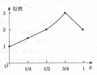
Parity and Variable Method

The method of scoring and the method of variing are the methods of obtaining subjective probabilities based on expert advice and then processing them into probabilities curves, which are actually a continuation of the notion of subjective probabilities.

The scoring method is the division of the possible range of parameters into equal lengths, and the inviting of experts in each small area to give subjective probabilities

The variation method is to divide all the zones into two sub-divisions of equal opportunity (no length of the zone) and experts need to give points.

We usually use the fractional method more so that we can better drive experts to think and give better answers.

With the division given by the experts, we can easily complete the construction of the probability histogram based on this information.

First, make sure you're a priori distributed and then determine the hyperparameter.

It's a very broad method.

Superparameter

We call the parameters in the aforecast distribution hyperparameter

In machine learning, the concept of hyperparameters is derived from Bayesian statistics, where parameters refer to the number that will be automatically determined during model learning, and superparameters refer to those that will need to be determined in advance in those models, so that the design of an automated superparameter adjuster will automatically determine the cross-reference.

And this section is the first one we're thinking of.$\theta$The a priori density is... $\pi(\theta)$ Among them are pending parameters $\mu$We're just gonna have to set this super-parameter behind us.$\mu$ I'll know about the a priori distribution.

Of course, it's easy to see. The core of this method is the selection of a priori distribution. $\pi(\theta)$ If this is the wrong place to choose, then the estimates will be very different.

Determine aforecast distribution

Based on the characteristics of the parameter space Parameter Space $(-\infty,\infty)$ Distribution: Normal distribution, Cosy distribution (average and variance not present), students $t$ Distribution, etc.; The distribution of parameter space (0, \infty) is: index distribution, Wable distribution, gamma distribution, etc.; Parameter Space $0,1,\ldots$ Distribution: Porcelain distribution, geometry, etc.;

Determine the hyperparameter

Rectangular estimate superparameters

The sample rectangles that were processed from the a priori information, and the equation that was used to determine the hyperparameters using the sample rectangulars equal to the total rectangulars, is the rectangular estimates, which are just used in the Bayesian statistics.

Estimated decimals

It's another idea of the super-parametrics.

We know that the overall fraction must be a function of the hyperparameter, and the sample fraction can be processed using sample information, and we can equalize the equation to determine the hyperparameter.

The score estimate is actually an important branch of classical statistics, but it is not presented in most mathematical statistics materials.

There are certainly more than two ways to determine the super-parameters than one, and we can estimate them together or use ideas from different mathematical statistics, such as those that are very similar.

Use a decimal to determine a priori CDF

If there is a greater a priori distribution of medians, it's like a proposed CDF curve, and the CDF curve, which is designed to reflect the a priori distribution, and the section of this paper "Standing with a Nuclear Density Curve" is close to thinking.

Use edge distribution

Marginal distribution lacks practical meaning, and the sampling of marginal distribution is theoretically possible, and in fact the knowledge of this subsection is less used in practical application

Marginal distribution

Definitions

We've been working on the definition of the margin distribution, and we've been working on this one. Section

When Random Variable$X$Probability density function$f(x|\theta)$ The pre-distribution density function is$\pi(\theta)$ can be defined as the distribution of random variables as $$00\ m\left(x\right)& =\int_{\Theta}f(x|\theta)\mathrm{d}F^{\pi}(\theta) \ &\left.=\left{\begin{array}{ll}\int_\Theta f(x|\theta)\pi(\theta)\mathrm{d}\theta,&\\theta\text{is a continuous random variable}, \\sum if(x\theta i)\pi(\theta i),&\theta\text{for discrete random variables}. \end{array}\right.\right.\right. I'm sorry, I'm sorry. The margin distribution is obtained by combining sample and a priori information.

Mixed distribution

When Random Variable$X$With probability.$p$Yes.$F({x|\theta_{1}})=F_{1}$Median Value $1-p$The probability is that$F({x|\theta_{1}})=F_{2}$We know that the combination is the only way to get a distribution. $X$The hybrid distribution function is$$F(x)=pF(x|\theta_1)+(1-p)F(x|\theta_2)$$ And it turns out that the distribution of the edges is actually a form of promotion of mixed distribution, a limitation.$\theta$For the discrete variable, the edge distribution is the result of a combination of probabilistic density functions.

When?$\theta$When the continuous variable is $m(x)$It's a mixture of infinity infinity.

An example of the calculation of the marginal distribution

Set Aspect$\theta$♪ A sample of time ♪$X$ Subject to normal distribution$N(\theta,\sigma^{2})$ of which$\sigma$Known.$\theta$A priori distribution is$N(\mu_\pi,\sigma_\pi^2)$ Calculate edge distribution$m(x)$ $$\begin{aligned} m(x)& =\int_{-\infty}^{\infty}f(x|\theta)\pi(\theta)\mathrm{d}\theta \ &=\frac{1}{2\pi\sigma\sigma_{\pi}}\int_{-\infty}^{\infty}\exp\left{\left.-\frac{1}{2}\left[\frac{(x-\theta)^{2}}{\sigma^{2}}+\frac{(\mu_{\pi}-\theta)^{2}}{\sigma_{\pi}^{2}}\right]\right}\mathrm{d}\theta\right. \ &=\frac{1}{2\pi\sigma\sigma_{\pi}}\int_{-\infty}^{\infty}\exp\left{-\frac{A}{2}\left(\theta-\frac{B}{A}\right)^{2}\right}\cdot\exp\left{-\frac{1}{2}\left(C-\frac{B^{2}}{A}\right)\right}\mathrm{d}\theta \ &=\frac1{\sqrt{2\pi(\sigma^2+\sigma_\pi^2)}}\exp\left{-\frac{(x-\mu_\pi)^2}{2(\sigma^2+\sigma_\pi^2)}\right} \end{aligned}$$ 其中 $$A=\frac{1}{\sigma^2}+\frac{1}{\sigma_{\pi}^2},\quad B=\frac{x}{\sigma^2}+\frac{\mu_{\pi}}{\sigma_{\pi}^2},\quad C=\frac{x^2}{\sigma^2}+\frac{\mu_{\pi}^2}{\sigma_{\pi}^2}$$ 也就是 $$N(\mu_\pi,\sigma^2+\sigma_\pi^2)$$

Or do you construct a density function with a final value of one, which is the classic method of processing the fractions in probability and statistics?

Perception Probability

Time of lapse of setting an electronic component $X$ Obedience index distribution $Exp(1/\theta)$, the density function is $f (x|theta)=\theta^-1}mathrm{e^-x/\theta}x>0)$, 若未知参数 $\theta$ 的先验分布为逆伽马分布 $\\Gamma^(1,100) calculates the probability that the component will expire on the edge before 200 hours. The probability of the edge is the fraction of the margin distributed between the corresponding zones. So the result of the calculations here is that $$\int_{0}^{200}m(x)dx =\frac{2}{3}$$

Select ML-II method for afore-distribution

Now, back to the point of this section, we're looking at a priori distribution selection, so let's talk about how to use the edge distribution to determine a priori distribution.

Our core thinking is still more likely to occur in the sample.

So we're going to select a priori distribution that gives the sample distribution a higher probability of the current situation.

Definitions and methods

Definitions: Set$\Gamma$ It's a priori class we're considering.$x=(x_{1},x_{2}...x_{n})$ If it exists $\hat{\pi}\in\Gamma$ Make $$m(\boldsymbol{x}|\hat{\pi})=\sup_{\pi\in\Gamma}\prod_{i=1}^nm(x_i|\pi)$$ Name$\hat{\pi}$The largest a priori for type II, or ML-II.

"In fact, it's a...$m(x)$Considers it a very, very a priori function) If the a priori density function is known to be just an unknown hyperparameter, then we can simplify the problem above to the following form, which is the one that we're looking at.$\Lambda$ It's a collection of values for hyperparameters. $$m(\boldsymbol{x}|\hat{\lambda})=\sup_{\lambda\in\Lambda}m(\boldsymbol{x}|\lambda)=\sup_{\lambda\in\Lambda}\prod_{i=1}^nm(x_i|\lambda)$$ That's the big, obvious question of studying our parametrics.$\Lambda$I'll take the value.

Why a bunch of serials? The margin distribution is calculated by the formula based on the base edge distribution for a sample of the margin distribution Of course, we can't have only one exterior distribution. We can understand it with a very specious idea of how to construct a function in a sample.

And simple random samples are naturally independent (i.i.d). The approximation is itself a series of probabilities and then it's dramatically increased. We usually call multiple multiplications. Joint Edge Density Function

Examples

Set Random Variables $X\sim N(\theta,\sigma^2)$, of which $\sigma^2$ Known, reset. $\theta\sim N(\mu_\pi,\sigma_\pi^2)$If... $X=(X_1,\cdots,X_n)$ To Distribution From Margins $m(x|\lambda)$ i.i.d. sample taken, test confirmed $\theta$ A priori distribution

First we'll study the distribution of the edges. $X$The distribution of the edges is$N(\mu_\pi,\sigma^2+\sigma_\pi^2)$ This paper, for example, "An example of the calculation of the distribution of the edges" section

According to the method before, we give the functions that we need to do to be radicalized.$\bar{x}$ and$S^{2}$The average and difference of the sample taken is $$00\ &L(\mu_\pi,\sigma_\pi^2|\boldsymbol{x}) =m(\boldsymbol{x}|\boldsymbol{\lambda}) \ & =\left[2\pi(\sigma^2+\sigma_\pi^2)\right]^{-n/2}\exp\left{-\frac{1}{2(\sigma^2+\sigma_\pi^2)}\cdot\sum_{i=1}^{n}(x_i-\mu_\pi)^2\right} \ &=\left[2\pi(\sigma^2+\sigma_\pi^2)\right]^{-n/2}\exp\left{\frac{-nS^2}{2(\sigma^2+\sigma_\pi^2)}\right}\cdot\exp\left{-\frac{n(\bar{x}-\mu_\pi)^2}{2(\sigma^2+\sigma_\pi^2)}\right}, \end{aligned}$$

It's easy to see. If$\sigma_{\pi}^{2}$- Fixed. - So...$\mu_{\pi}=\bar{x}$When you're trying to maximize it, you don't need to be partial.

Bring in$\mu_{\pi}=\bar{x}$ $$\phi(\sigma_{\pi}^{2})=\big[2\pi(\sigma^{2}+\sigma_{\pi}^{2})\big]^{-n/2}\exp\bigg{\frac{-nS^{2}}{2(\sigma^{2}+\sigma_{\pi}^{2})}\bigg}.$$ The logarithmic guidance study was extremely successful. $$\hat{\sigma}_\pi^2=S^2-\sigma^2$$ Obviously, it's impossible to take the burden.$S^{2}$When I was little.$0$Yeah.

Select the rectangular method for a prior distribution

The core here is to study the relationship between the margin distribution and the a priori distribution rectangular, so that the rectangular estimates of the a priori distribution parameters are achieved by a sample of reality, and the prior direct study of the a priori rectangular estimates are different, and at this point we lack direct knowledge of the a priori.

The core idea is to estimate the edge distribution rectangular, which is a function of the margin distribution rectangular.

Theory leads

Calculate sample distribution$f(x|\theta)$The expectations and the differences.$\theta$It's a constant, yeah.$x$The hope is different from the difference) $$\mu(\theta)=E^{X|\theta}(X),\quad\sigma^{2}(\theta)=E^{X|\theta}[X-\mu(\theta)]^{2},$$ Calculate edge distribution$m(x)=m(x|\lambda)$Expectations and differences$\lambda$(overparameters) is constant pair$x$The hope is different from the difference)

$$\begin{aligned} &\mu_{m}(\lambda) =E^{X|\lambda}(X)=\int_{\mathcal{C}}xm(x|\lambda)\mathrm{d}x=\int_{\mathcal{C}}\int_{\Theta}xf(x|\theta)\pi(\theta|\lambda)\mathrm{d}\theta\mathrm{d}x \ &=\int_\Theta\left[\int_{\mathscr{E}}xf(x|\theta)\mathrm{d}x\right]\pi(\theta|\lambda)\mathrm{d}\theta=\int_\Theta\mu(\theta)\pi(\theta|\lambda)\mathrm{d}\theta \ &=E^{\theta|\lambda}[\mu(\theta)], \ &\sigma_{m}^{2}(\lambda) =E^{X|\lambda}\left{[X-\mu_{m}(\lambda)]^{2}\right}=\int_{\mathcal{E}}[x-\mu_{m}(\lambda)]^{2}m(x|\lambda)\mathrm{d}x \ &=\int_{\mathscr{X}}\int_{\Theta}[x-\mu_m(\lambda)]^2f(x|\theta)\pi(\theta|\lambda)\mathrm{d}\theta\mathrm{d}x \ &=\int_{\Theta}\left{\int_{\mathscr{X}}[x-\mu_{m}(\lambda)]^{2}f(x|\theta)\mathrm{d}x\right}\pi(\theta|\lambda)\mathrm{d}\theta \ &=\int_{\Theta}E^{X|\theta}\left[x-\mu_{m}(x)\right]^{2}\pi(\theta|\lambda)\mathrm{d}\theta, \end{aligned}$$ 其中 $$\begin{aligned} &E^{X|\theta}\left{\left[x-\mu_m(\lambda)\right]^2\right} =E^{X|\theta}\left(\left{\left[x-\mu(\theta)\right]+\left[\mu(\theta)-\mu_{m}(\lambda)\right]\right}^{2}\right) \ &=E^{X|\theta}\left{\left[x-\mu(\theta)\right]^2\right}+E^{X|\theta}\left{\left[\mu(\theta)-\mu_m(\lambda)\right]^2\right} \ & =\sigma^2(\theta)+\left[\mu(\theta)-\mu_m(\lambda)\right]^2. \end{aligned}$$ 因此方差实际上的表示为 $$\begin{gathered} \sigma= (m)= (m)= (m)= (m)= (m)= (m)= (m)= (m)= (m)= (m)= (m)= (m)= (m){ (m){ (m){ (m){ (m){ (m){ (m){ (m){ (m){ (m){ (m){ (d)\theta{ (m){ (m){ (m){ (m){ (m){ (m){ (m){ (m){ (m){ (m){ (m){ (m){ (m){ (m){ (m){ (m){ (m){ (m){t){ (m){t){ (m){tta){ (m){ta (m){tta){ (m){ (m) (m) (m){tta){ (m) (m) (m) (m) (m) (m) ♪ It's a good thing you're not a good guy ♪ I'm sorry, I'm sorry. Parameters here$\lambda$It's a generic description of the parameters in the aforethought distribution, not just the parameters.

If we're only two super-parameters in a priori distribution, $\lambda_{1},\lambda_{2}$ So the rectangular estimate only takes two volumes, which is easy to calculate for two margin distribution rectangles (the most basic expectations and the difference) What's that?{m}=\overline{X}=\frac{1}{n}\sum♪ I'm not gonna let you go ♪{m}^{2}=S^{2}=\frac{1}{n-1}\sum{i=1}^{n}(X_{i}-\overline{X})^{2}$$

The equation of the extricated sample rectangular has the results we need to know about the hyperparameter. $$\left.\left{\begin{array}{l}\hat{\mu}_m=E^{\theta|\boldsymbol{\lambda}}\big[\mu(\theta)\big],\\hat{\sigma}_m^2=E^{\boldsymbol{\theta}|\boldsymbol{\lambda}}\big[\sigma^2(\theta)\big]+E^{\boldsymbol{\theta}|\boldsymbol{\lambda}}\big[\mu(\boldsymbol{\theta})-\mu_m(\boldsymbol{\lambda})\big]^2\bigg}.\end{array}\right.\right.$$

Language expression of the final formula:

• Estimates of the margin distribution average: we calculate the sample distribution average for parameters$\lambda$ Expectations
• Estimates of differentials in the margin distribution: the difference in the sample distribution is about parameters$\lambda$ The expectations and the sample distribution averages about the parameters$\lambda$ the difference between

The averages and the differences in the sample distributions are their own, and they're their parameters.$\lambda$That's the principle of calculation.

Examples

Set $X|\theta\sim N(\theta,1)$,parameters $\theta$ A priori distribution to $N(\mu_\pi,\sigma_\pi^2)$, of which $\lambda=(\mu_\pi,\sigma_\pi^2)$ Unknown. $X=(X_1,\cdots,X_n)$ To Distribution From Margins $m(x|\lambda)$ i.i.d. sample from which the sample is calculated as the average sample value $\bar{X}=10,S^{2}=3.$ Try to be sure. $\theta$ A priori distribution

Study using rectangular estimation

The expected distribution and the difference in the sample distribution are different $\theta$ and $1$

The expectations and differences in calculating the marginal distribution are: $$\left.\left{\begin{array}{l}\mu_m(\lambda)=E^{\theta|\lambda}(\theta)=\mu_\pi,\\sigma_m^2(\lambda)=E^{\theta|\lambda}(\sigma^2(\theta))+E^{\theta|\lambda}[\theta-\mu_\pi]^2=1+\sigma_\pi^2.\end{array}\right.\right.$$

Average and variance of the sample taken into the sample $$\left.\left{\begin{array}{l}10=\overline{X}=\mu_\pi,\3=S^2=1+\sigma_\pi^2.\end{array}\right.\right.$$ And so...$\theta$The a priori distribution is$N(10,2)$

No information a priori distribution

The Beyers statistics are characterized by the use of a priori information in statistical extrapolation.

But sometimes, there's little or no information, and we still want to use the Beyers statistics idea.No information a priori (noninformation preor) is that there is no preference for any parameter space at all

Bayesian hypothetical and broad a priori distribution

No information a priori distribution means our a priori distribution does not contain any$\theta$There is no preference for any value in the information.

Definitions

It's natural. We can put it in.$\theta$As a flat distribution in the range of values taken, it is considered a priori distribution, which is the Bayes assumption, which usually follows:

• Disperse evenly if$\Theta$ It's a limited set, so the dispersive distribution is evenly distributed. $P(\theta=\theta_i)=1/n$
• A limited area is evenly distributed if$\Theta$ It's a limited area.$[a,b]$ So the limited area is evenly distributed$U(a,b)$
• Broad a priori distribution if$\Theta$ - No bounds. - So?$\pi(\theta)\equiv1$ He doesn't meet probabilistic criteria, so it's broad.

Definitions: If$\theta$A priori distribution$\pi(\theta)$ Satisfied

• $\pi(\theta)\equiv1$ And...$\int_{\Theta}\pi(\theta)\mathrm{d}\theta=\infty;$
• Post-density$\pi(\theta|x)$It's normal density function. And then, "Could"$\pi(\theta)$ Yes.$\theta$ Broad a priori density (improper prier density)

It's easy to know whether a priori density is broad enough to multiply any constant or a priori density is broad enough to be a priori.

Bates' hypothesis is not enough.

The Beyers hypothesis is a disadvantage, the biggest one being uncertainty.

If we're right...$p$I'm equally ignorant.$p^2,p^3$So, theoretically, we take the Bayesian hypothesis.$U(0,1)$The distribution of the three of them should not change; obviously, in many cases it is not.

Bates' assumption is not enough for the change of the constant. For example: consider normal standard deviations $\sigma\in(0,\infty)$, define a change $$ \eta=\sigma^2\in(0,\infty) $$ then $\eta$ Normal difference Set $\sigma$ The a priori density function is $\pi(\sigma)$, $\eta$ A priori density function is $\pi^(\eta)$, 那么$The \eta$ density function can be expressed as $$$2 million(\eta)=\pi(\sqrt{\eta})\left|\frac{d\sigma}{d\eta}\right|$$

As you can see, you cannot set a constant for a priori distribution of a parameter, which means that the Bayesian hypothesis cannot be used at random.

No information a priori for the position parameter family

General $X$ . The density function is as follows: $f(x-\theta)$, its sample space $\mathscr{X}$ and parameter space $\Theta$ The distribution of these density functions is called the positional parameter group (localization modeler family), and the location function is a series of sites that are located in the country. $\theta\in\Theta$ Called position parameters.

Here are two examples of the two position parameter communities. Normal distribution $$\frac{1}{\sqrt{2\pi}\sigma}\exp\Big{\frac{1}{2\sigma^2}(x-\theta)^2\Big}=f(x-\theta)$$ Couchy distribution $$\frac1\pi\cdot\frac\lambda{\lambda^2+(x-\mu)^2}=f(x-\mu)$$

It's easy to see that the position parameter community is not in the same shape as the lateral variant.

Yeah.$X$I can do the transposition. $Y=X+c$ And also against arguments$\theta$I can do the transposition. $\mu=\theta+c$ It's easy to know. $Y$The density function is as follows: $f(y-\mu)$ Or is it a member of the position parameter community and the sample space and parameter space is unchanged?

So the statistical problems of both studies are the same, and we should think they have the same no-information a priori, and we'll go to prove that no-information a priori density is the same.$\pi(\theta)\equiv1$

You! $\pi$ And $\}$ 分别表示 $\theta$ 与 $\eta$ 的无信息先验密度，以上论点说明 $\pi$ 和 $\pi^{It should have the same a priori density, that is $ \ pi (\ pi)= pi^(\tau)$$ 由于前面的线性关系我们知道 $$\pi(\eta)=\pi^(\eta)=\pi(\eta-c)$$ 特别的 我们取$\eta=c$ $$\pi(c)=\pi(0)=\text{ constant}.$ So we take it.$\pi(\theta)\equiv1$ It's reasonable. I'm not sure what I'm talking about.$\theta$ When a position parameter is not previously obtained as constant or 1

No information a priori for the spectrometers

General $X$ . The density function is as follows: $\sigma^{-1}\varphi(x/\sigma)$,$\sigma of which>0$ 为刻度参数，参数空间为 $\matbb{R} + (0, \infty) $, and the distribution of these density functions is called the scale parameter family

Here are a few examples. Normal distribution with an average of 0 $$00\ f (x|sigma)& =\frac1{\sqrt{2\pi}\sigma}\exp\left{-\frac{x^2}{2\sigma^2}\right} \ &=\sigma^{-1}\left[\frac1{\sqrt{2\pi}}\exp\Big{\left.-\frac12\left(\frac x\sigma\right)^2\right}\right]=\sigma^{-1}\varphi\Big(\frac x\sigma\Big), \end{aligned}$$ 伽马分布 $$f(x|\lambda)=\frac{\lambda^{-r}}{\Gamma(r)}x^{r-1}\mathrm{e}^{-x/\lambda}=\lambda^{-1}\Big[\frac{1}{\Gamma(r)}\Big(\frac{x}{\lambda}\Big)^{r-1}\mathrm{e}^{-x/\lambda}\Big]=\lambda^{-1}\varphi\Big(\frac{x}{\lambda}\Big),$$

And the same principle, which shows the constantity of the tic parameter family in the tics.

Yeah.$X$Change $Y=cX$ Yeah.$\theta$Make the corresponding changes $\eta=c\sigma$ Got it.$Y$ Or a member of the spectroparameters, so it's reasonable for both to choose the same as the non-information a priori.

According to the same means of proof as before, we take $$\ (\sigma)=firc1}{\sigma=>(0) $ Uninfoted aforecast distribution as a symmetric parameter family

Position-scale parameter family

Let's take a position-scale parameter in the context of the previous text. Group

Set density functions with two parameters $\mu$ and $\sigma$, and density takes the following forms: $$ p(x;\mu,\sigma)=\frac1\sigma f\left(\frac{x-\mu}\sigma\right),\mu\in(-\infty,\infty),\sigma\in(0,\infty) $$ of which $f( x)$ Is a fully established function, $\mu$ Called position parameters,$\sigma$ Called a measure parameter, and this sort of distribution group called a position-scale parameter Group

The normal distribution, the Cauchy distribution, the index distribution, is evenly distributed in this category.

I am not sure if I am.$\sigma=1$ is often called the position parameter, and$\mu=0$ The current term is the scale parameter family, the position-scale parameter group being the combination of the two above

His counterpart's no information a priori. $\pi(\theta,\sigma)=\frac{1}{\sigma^{2}}$

General Uninformation Precursion

The uninfomatic a priori of the general situation is the most common method of Jeffreys, because its extrapolation involves a lot of information about abstract algebra variations and Harr measurements, and we will only present the method below.

Jeffreys has no information a priori.

Assumptions for sample distribution ${f(x|\theta),\theta\in\Theta}$ Meet CR. $\theta=(\theta_1,\cdots,\theta_p)$ Yes $p$ Width vector. Set $\boldsymbol{X}=(X_1,\cdots,X_n)$ From the whole. $f(x|\theta)$ Simple sample taken. When?$\theta$ When no a priori information is available, Jeffreys uses the square root of the Fisher Info array in a row $\theta$ ..no information a priori called

Jeffreys has no information to solve the problem.

1. Write Parameters$\theta$logarithmic function $$l(\boldsymbol{\theta}|\boldsymbol{x})=\ln\left[\prod_{i=1}^nf(x_i|\boldsymbol{\theta})\right]=\sum_{i=1}^n\ln f(x_i|\boldsymbol{\theta}).$$
2. Calculating Fisher Information Frame $I (\bardsymbol(theta}) =\left(I ij}(\bardsymbol(theta})\right){p\times p},\quad I{ij}(\boldsymbol{\theta})=E_{\boldsymbol{X}\mid\boldsymbol{\theta}}\Big{-\frac{\partial^2l}{\partial\theta_i\partial\theta_j}\Big}\quad(i,j=1,\cdots,p).$$ For a single parameter scenario Fisher Info array is$1\times1$Matrix $$I(\boldsymbol{\theta})=E_{\boldsymbol{X}|\boldsymbol{\theta}}\Big{-\frac{\partial^{2}l}{\partial\boldsymbol{\theta}^{2}}\Big}.$$ Take this down.$E$- Yeah.$X$It's good. There's got to be a sample in there.
3. The square root of the column of the Calculating Info array as a priori without information $$\pi(\theta)=\left[\det I(\theta)\right]^{1/2}$$ For a single parameter situation $$\pi(\theta)=[I(\theta)]^{1/2}.$$

Fisher's Information Volume Definition is $$I(\theta)=E_\theta\left[\frac\partial{\partial\theta}\ln p(x;\theta)\right]^2$$ The form we're using above is a price equivalent that meets the notion of a detailed study of Fisher's information volume, which will give us a detailed description of the definition and the reasoning. If you don't stress the number of samples, you should take only one sample, if the number of samples is not good.

Examples

Set $X=(X_1,\cdots,X_n)$ From the whole. $N(\mu,\sigma^2)$ Simple sample taken. Remember$\theta=(\mu,\sigma)$Please. $(\mu,\sigma)$ Joint without aforeword

The calculation logarithmic function is as if $$l(\boldsymbol{\theta}|\boldsymbol{x})=-\frac n2\ln2\pi-n\mathrm{ln}\sigma-\frac1{2\sigma^2}\sum_{i=1}^n(x_i-\mu)^2.$$ The elements of the Fisher Info-Founding for Division $$00begin{aligned}I 11(\bardsymbol{\theta}&=E_{\boldsymbol{X}|\boldsymbol{\theta}}\Big{-\frac{\partial^2l(\boldsymbol{\theta}|\boldsymbol{x})}{\partial\mu^2}\Big}=\frac{n}{\sigma^2},\I_{22}(\boldsymbol{\theta})&=E_{\boldsymbol{X}|\boldsymbol{\theta}}\Big{-\frac{\partial^2l(\boldsymbol{\theta}|\boldsymbol{x})}{\partial\sigma^2}\Big}=-\frac{n}{\sigma^2}+\frac{3}{\sigma^4}E\Big{\sum_{i=1}^n(X_i-\mu)^2\Big}=\frac{2n}{\sigma^2},\I_{12}(\boldsymbol{\theta})&=I_{21}(\boldsymbol{\theta})=E_{\boldsymbol{X}|\boldsymbol{\theta}}\Big{-\frac{\partial^2l(\boldsymbol{\theta}|\boldsymbol{x})}{\partial\mu\partial\sigma}\Big}=E\Big{\frac{2}{\sigma^3}\sum_{i=1}^n(X_i-\mu)\Big}=0,\end{aligned}$$ 计算Fisher信息阵和行列式的平方根有 $$\left.I(\boldsymbol{\theta})=\left(\begin{array}{cc}\frac n{\sigma^2}&0\0&\frac{2n}{\sigma^2}\end{array}\right.\right),\quad[\det I(\boldsymbol{\theta})]^{1/2}=\frac{\sqrt{2}n}{\sigma^2}.$$ 由于广义先验可以自由调整常数 联合无信息先验为 $$\pi(\mu,\sigma)=1/\sigma^2,$$

Or this example, we can see.

When?$\sigma$When known, belonging to the position parameter family, no information a priori should read$\pi(\theta)\equiv1$ The fact that the Felher information array was used to calculate Jeffreys' lack of information a priori is the same result.

When?$\mu$When known, the data should be \pi(\sigma) = \frac{1}{\sigma}\quad(\sigma)>This is also the result of the fact that Jeffreys' lack of information was calculated using Fisher's Info array.

So when they were independent, the joint no-information aforema density was $\pi(\sigma)=\frac{1}{\sigma}\sigma>(0) When they're not independent, no information is combined a priori density$\pi(\mu,\sigma)=1/\sigma^2,$

I can see that. No information a priori density is not unique

In fact, the impact of the different information a priori on the Bayesian inference is small.

The absence of information a priori is one of the most successful parts of Bayesian statistics.

Many of the estimates in classical statistics can be considered as some kind of anaesthesia without information.

Co-examining distribution

It's a theoretical way of determining a priori, and in the case of known samples, for theoretical research purposes.

In fact, the distribution of the edges in the high-dimensional context is very difficult to calculate.

Definitions

Definitions$\mathscr{F}$ Other Organiser $\theta$ A priori distribution $\pi(\theta)$ Composition of the distributed community. If you're willing to take it,$\pi\in\mathscr{F}$ and sample values $x$,Performing Distribution$\pi( \theta|x)$ Still belongs to $\mathscr{F}$ So, what do you say? $\mathscr{F}$ A co-prospective distribution (conjugate prefix distribution family)

It's obvious that the a priori values of the distributional and sampled are relevant.

At the same time, the a priori distribution is for one parameter in the distribution, and it is important to understand the circumstances that contain multiple parameters.

Examples of co-prospecting distributions

Set$X\sim B(n,\theta)$

• If $\theta$ Obedience evenly distributed $U(0,1)$, attests: $\theta$ The posteriori distribution is the Beta distribution;
• If $\theta$ A priori distribution is the beta distribution $Beta(a,b)$, of which $a,b$ Known, attests to: $\theta$ The posteriori distribution is still the Beta distribution, i.e. $\theta$ The co-prospecting distribution is the Beta distribution.

Two questions in a row are really a question of a posteriori distribution.

1. The following is the text: Sample distribution is in two forms: $$f(x|\theta)=\binom nx\theta^x(1-\theta)^{n-x}\quad(x=0,1,\cdots,n)$$ The aforecast distribution is evenly distributed $\pi(\theta)=1$ The post-calculation distribution is as follows: $$\pi(\theta|x)=\frac{\theta^x(1-\theta)^{n-x}}{\int_0^1\theta^x(1-\theta)^{n-x}\mathrm{d}\theta}$$ Calculating the points is the mathematical analysis of the Gamma function's points. Pass. $$\int_0^1\theta^x(1-\theta)^{n-x}\mathrm{d}\theta=\frac{\Gamma(x+1)\Gamma(n-x+1)}{\Gamma(n+2)}.$$ So they get a posteriori distribution. $$\pi(\theta|x)=\frac{\Gamma(n+2)}{\Gamma(x+1)\Gamma(n-x+1)}\theta^{(x+1)-1}(1-\theta)^{(n-x+1)-1}$$

2. The following is the text: The sample distribution is unchanged, the pre-specification distribution is Beta, and the same principle is applied to the post-calculation distribution. $$\pi(\theta|x)=\frac{\theta^{x+a-1}(1-\theta)^{n-x+b-1}}{\int_0^1\theta^{x+a-1}(1-\theta)^{n-x+b-1}\mathrm{d}\theta}$$ And we're going to calculate the points and bring in the results and we're going to have a back-up density. $$\pi(\theta|x)=\frac{\Gamma(n+a+b)}{\Gamma(x+a)\Gamma(n-x+b)}\theta^{(x+a)-1}(1-\theta)^{(n-x+b)-1}$$ So we're sure it's a co-prospecting distribution.

Determine the distribution after co-checking

We can think of a sample.$X$..the density of the edge$f_{m}(x)$ and$\theta$It's not about that, which means he's a constant. $$\pi(\theta|x)=\frac{f(x|\theta)\pi(\theta)}{f_m(x)}\propto f(x|\theta)\pi(\theta)$$

Definition: The kernel of the probability function is the part of the probability function that is only relevant to the parameters *Eg. Sample Probability Functions$f(x|\theta)$- The core. - Yes.$f(x|\theta)$only with$\theta$Relevant part

For co-prospecting distributions, the following steps can be taken to test back density:

1. Write sample probability function$f(x|\theta)$. . . . . . . . . and pre-density functions $\pi(\theta)$ Nuclear
2. Using the formula at the end of the line, you give back-density cores, which are the mass of sample cores and a priori sum.
3. Add a regular constant factor and get a posteriori density.$x$(Refer to)

How to add a regular constant factor: the distribution of the back-density of co-scoping is known. We can just go to the corresponding back-density function.

This method is generally only available for a priori distribution.

Because we know that the back check is the same as the a priori density function, and we know the distribution of the back check is easy to give constants.

When a non-cooperative aforesee, but a later check, we know that it's a core of a common distribution, and it can be given.

In other cases, we can't determine the constant factor, but we need to calculate it according to the basic formula of the later check.

Specific examples can be found in the section “Accounting for later distribution” of this paper

Multi-layer a priori (phased a priori)

Basic thinking

If the parametric parameter is not certain, then the second is called superprecursor, and if it's still difficult to determine whether we can continue the pre-precursion, the new a priori is called multi-layer a priori based on a priori and superpresence.

The multilayered aforethought is as follows: First level a priori $F_1={\pi_1(\theta|\lambda):\pi_1$. . . . . . . . . . . . . . . . . . . . . . . . . . . . . . . . . . . . . . . . . . . . . . . . . . . . . . . . . . . . . . . . . . . . . . . . . . . . . . . . . . . . . . . . . . . . . . . . . . . . . . . . . . . . . . . . . . . . . . . . . . . . . . . .$\lambda\in\Lambda}$I'm not sure. of which $\Lambda$ As Superparameter $\lambda$ range of values to be taken from, and λ unknown

Second floor a priori. $\lambda$The a priori distribution is$\pi(\lambda)$ Without any unknown parameters

The two levels of the calculation code are pre-established $$\pi(\theta)=\int_{\Lambda}\pi_1(\theta|\lambda)\pi_2(\lambda)\mathrm{d}\lambda=\int_{\Lambda}\pi(\theta,\lambda)\mathrm{d}\lambda$$

The core is to get our standard a priori distribution through multilayered compound a priori, and then use this standard a priori distribution for the Bayesian statistical extrapolation.

Pre-specify the stratification

To study the a priori distribution of the failure rate, we first consider the failure rate to be a priori.$U(0,1)$ But the failure rate is low, so this a priori is not a reasonable one, so it's a choice to use multilayer a priori to study it.

We think the failure rate is... $U(0,\lambda)$ of which super-parameters$\lambda$A priori as$U(0.1,0.5)$

Calculates a priori for regularization. $$\pi(\theta)=\int_{\Lambda}\pi_{1}(\theta|\lambda)\pi_{2}(\lambda)\mathrm{d}\lambda=\frac{1}{0.5-0.1}\int_{0.1}^{0.5}\lambda^{-1}I_{[0,\lambda]}(\theta)\mathrm{d}\lambda$$ of which$I$is a specter function that calculates a priori results in several different cases.

$$\begin{aligned}&(a)\text{bet }0<\theta<..the time of the ..&\pi\left(\theta\right)=\frac{1}{0.4}\int_{0.1}^{0.5}\lambda^{-1}d\lambda=2.5\ln5\approx4.0236;\end{aligned}$$ $$\begin{aligned}&\text{b) \leqslant\theta<0.5\text{t}, \\&\pi\left(\theta\right)=\frac{1}{0.4}\int_{\theta}^{0.5}\lambda^{-1}d\lambda=2.5\left(\ln\left(0.5-\ln\theta\right)\approx-1.7329-2.5\ln\theta\right);\end{aligned}$$ $$(c) \\theta\geqslant0.5, \\theta)=$0.00

All right, all right. $$\left.\pi(\theta)=\left{begin{array}ll}4.0236,&0<\theta<0.1,\-1.7329-2.5\ln\theta,&0.1\leqslant\theta<0.5,\0,&0.5\leqslant\theta<I'm sorry, I'm sorry, but I'm sorry. Just to meet the normative requirements of the probabilistic density function

A priori ideological characteristics of the hierarchy

A priori stratification model allows for the conversion of relatively complex situations into a series of cartridges when modelling As we have seen in the preceding example, although we are still making a stratification a priori norm, the stratification Beyers model allows us to decompose relatively complex situations into a series of simple situations that make modelling less difficult. Sometimes our norms are complicated to the point where they don't even have a visible expression, but the layers of Bayes still help us to model.

Another feature of the stratification a priori model is that it is easy to calculate. Sometimes the posterior density is too complicated, which makes it difficult to calculate him and some of his digital features, and leads to the Beyers statistical inferences that statistical decisions are difficult to make. But if we use the hiercurate of multi-layer structures to indicate laterals, even if the outer layer is not represented by the expression, we can calculate it using methods like MCMC.

Co-prospecting of the index distribution

The necessary description of the mathematical statistics of the index distribution is given.Mathematical statistics and the “Indicate distribution” section

Co-a prior distribution of single-parameter index distributions

If $X|\theta$ The distribution is of an indexed group (samples distribution): $x=(x_1,\cdots,x_n)$ The sample is i.i.d. The apparent function can be expressed as $$ l(\theta|x)\propto[h(\theta)]^n\exp\left{\sum_{i=1}^nt(x_i)\phi(\theta)\right} $$ That is, the index distribution family parameter $\theta$ The Co-Protesters $\Pi$ Yes $\pi(\theta)$ Is: (Use of co-prospecting density functions to give the same form as the density functions of the sample) $$ \pi(\theta)\propto[h(\theta)]^{\gamma}\exp{{\tau\phi(\theta)}} $$ of which super-parameters $\gamma,\tau$ Known.

Co-prospective distribution of the two parameter index distributions

If $x=(x_1,\cdots,x_n)$ For the i.i.d. sample,$X$ , which is an index distribution family with two parameters, is an approximation $l(\theta,\varphi|x)$ May be read: $$ l(\theta,\varphi|x)\propto[h(\theta,\varphi)]^n\exp\left{\sum[t(x_i)\phi(\theta,\varphi)]+\sum[u(x_i)\chi(\theta,\varphi)]\right} $$ Parameters $(\theta,\varphi$ A priori. $\Pi$ Is this the following: $$ \pi(\theta,\varphi)\propto[h(\theta,\varphi)]^\gamma\exp\left{\alpha\phi(\theta,\varphi)+\beta\chi(\theta,\varphi)\right} $$ of which super-parameters $\gamma,\alpha,\beta$ Known

Multiparameter model

The idea of a multiparametric model

The idea of solving the backsizing of a given parameter has been described before.

The basic idea is to give a priori and then use formulas to make a later calculation.

In a large number of practical questions, it is common to have multiple unknown parameters, and we can give a back-sizing by a method similar to the single parameter.

Sometimes we focus on only a fraction of all the parameters, and at this point, to get the marginal back-density of the parameters that we're interested in, we need to get a fraction of the whole back-density of the parameters.

Examples of multiparametric models

The government has also been able to provide information on the situation.$\underline{x}=(x_1,\cdots,x_n)$ As Sample Capacity with$n$ i.i.d sample, unknown parameter $(\theta,\sigma^2)$ for a 2-D random variable, if$(\theta,\sigma^2)$ A priori density is $\pi(\theta,\sigma^2)\propto\frac1{\sigma^2}$,

$(1)\left(\theta,\sigma^{2}\right)|x$ Joint Postdensity Function $\pi(\theta,\sigma^2|x)$ Is: $$ \pi(\theta,\sigma^2|x)\propto(\sigma^2)^{-\frac{\gamma+1}2-1}\exp\left{-\frac1{2\sigma^2}\left(S+n(\bar{x}-\theta)^2\right)\right} $$ of which $\gamma=n-1,:S=\sum_{i=1}^{n}\left(x_{i}-\bar{x}\right)^{2},:\bar{x}=\frac{1}{n}\sum_{i=1}^{n}x_{i}$

(2) $\theta$ The marginal lateral distribution is:

$$ t=\frac{\theta-\bar{x}}{s/\sqrt{n}}\sim t(\gamma) $$ of which $s^2=\frac1{n-1}S$, $t(\gamma)$ It's freedom. $\gamma$ Yes. $t$ Distribution

(3) Difference $\sigma^2$ Other Organiser $$00\ \pi (sigma^)& =\int\pi(\theta,\sigma^{2}|x)d\theta \ &=\int_{-\infty}^{+\infty}\left(\sigma^2\right)^{-\frac{\gamma+1}2-1}\exp\left{-\frac1{2\sigma^2}\left(S+n(\theta-\bar{x})^2\right)\right}d\theta \ &\propto\left(\sigma^{2}\right)^{-\frac{\gamma}{2}-1}\exp\left{-\frac{S}{2\sigma^{2}}\right} \ &\times\int_{-\infty}^{+\infty}\left(\frac{2\pi\sigma^2}n\right)^{-\frac12}\exp\left{-\frac1{2\sigma^2}\cdot n(\theta-\bar{x})^2\right}d\theta \ &== sync, corrected by elderman == I'm sorry, I'm sorry. The equation to the right is the reverse of Gamma distribution core, so the difference is $\sigma^2$ The after-check margin distribution is$IGamma(\frac{\gamma}{2},\frac{S}{2})$

Calculation of the posteriori distribution

Calculation of the posteriori distribution

Theory Introduction

The calculations of the post-spectrum distribution are the basis for all the Beyers statistical inferences.

The formula for the posteriori distribution is: $$\pi(\theta|x)=\frac{h(x,\theta)}{m(x)}=\frac{f(x|\theta)\pi(\theta)}{\int_{\Theta}f(x|\theta)\pi(\theta)\mathrm{d}\theta}$$ Which means we need to make a score for the edge distribution.

This step is not always a good measure.

Common Post-Assessment Method

We have three ways of calculating the posteriori distribution.

• General calculation based on the Bayesian formula: definition of a later distribution
• Simplified calculation method based on distribution nuclear
• Calculation methods based on adequate statistical data There are two types of pre-selection that are more common.
• No information a priori distribution
• Co-examining distribution

Examples of calculations for the posteriori distribution

Example 1

We're still counting the front set.$X\sim B(n,\theta)$ $\theta$ A priori distribution is the beta distribution $Beta(a,b)$ Sample density core$\theta^x(1-\theta)^{n-x}$ The pre-density core is $\theta^{a-1}(1-\theta)^{b-1}$ So the posterioris content is satisfied. $$\pi(\theta|x)\propto f(x|\theta)\pi(\theta)\propto\theta^{x+a-1}(1-\theta)^{n-x+b-1}.$$ Apparently, he's also a beta distribution core, with a positive factor to supplement Beta distribution. $$\pi(\theta|x)=\frac{\Gamma(n+a+b)}{\Gamma(x+a)\Gamma(n-x+b)}\theta^{(x+a)-1}(1-\theta)^{(n-x+b)-1}$$

Example 2

Set$X$Subject to normal distribution$N(\theta,\sigma^{2})$ The difference is known, but the average is unknown.$\theta$The a priori is...$N(\mu,\tau^2)$ All parameters are known. $$\pi(\theta|x)\propto f(x|\theta)\pi(\theta)\propto\exp\left{-\frac{1}{2}\Big[\frac{(x-\theta)^2}{\sigma^2}+\frac{(\theta-\mu)^2}{\tau^2}\Big]\right}.$$ You! $$\rho=\frac{1}{\tau^{2}}+\frac{1}{\sigma^{2}}=\frac{\sigma^{2}+\tau^{2}}{\sigma^{2}\tau^{2}}.$$ Simpliciting the squared construction $$\pi(\theta|x)\propto\exp\Big{-\frac\rho2\Big[\theta-\frac1\rho\Big(\frac\mu{\tau^2}+\frac x{\sigma^2}\Big)\Big]^2-\frac{(x-\mu)^2}{2(\sigma^2+\tau^2)}\Big}\propto\exp\Big{-\frac{\rho}{2}\Big[\theta-\frac{1}{\rho}\Big(\frac{\mu}{\tau^{2}}+\frac{x}{\sigma^{2}}\Big)\Big]^{2}\Big}$$ I can see that. $N(\mu(x),\eta^{2})$ ..to add a regularised factor to the core to obtain a post-feasibility. $$\pi(\theta|x)=\frac{1}{\sqrt{2\pi}\eta}\exp\Big{-\frac{1}{2\eta^2}[\theta-\mu(x)]^2\Big}.$$ of which $$\begin{aligned}\mu(x)&=\frac{1}{\rho}\left(\frac{\mu}{\tau^2}+\frac{x}{\sigma^2}\right)=\frac{\sigma^2}{\sigma^2+\tau^2}\mu+\frac{\tau^2}{\sigma^2+\tau^2}x,\\eta^2&♪ I'm not gonna let you go ♪ When the sample is distributed to the known normal distribution of the variance, the mean parameter is$\theta$The co-prospecting distribution is normal.

Example 3

And here we give some examples of co-prospecting distribution, not counting, but simply giving some examples.

• Sample distribution is Porpine distribution$P(\theta)$And then, if the density is in line with the gamma distribution, then the later distribution is in the gamma distribution, which is the co-prospecting distribution group is in the gamma distribution.
• The sample distribution is gamma. $\Gamma(r,\lambda)$ of which$r$Known$\lambda$The co-prospecting distribution is the gamma distribution.
• The index distribution is a special case of gamma distribution, so the sample distribution is as follows:$Exp(\lambda)$♪ When ♪ $\lambda$The co-prospecting distribution is the gamma distribution.
• The difference is when the sample distribution is the known normal distribution of the average.$\sigma^{2}$The co-prospecting distribution is anti-Gamma distribution.

Brief summary

There's a fixed idea to be made of the distributional community.

1. Writes the core of the sample probability function
2. The probability function for selecting a nuclear sample has a priori distribution of the same core (in similar forms) as a co-prospecting distribution, and thus a co-prospecting distribution.

The nuclear of the probability density of the sample, which contains$\theta$, but at this point we're distributed$X$It's given as a variable if we put$\theta$It's a self-variant. He's supposed to be another distribution core.

I can see that.

• Co-examining distribution is easy to calculate and then distribute.
• There are many parameters for a posteriori distribution that can be explained very well.

For example, in the case of the normal distribution, the average after-checking was determined by a priori and sample, and as the amount of sample information increased, the role of the precursor was weakened by nature.

We then turn to the section on "Assumption and sufficiency" of a method that uses sufficient statistical data and the section on "Beyers statistical calculations" of a numerical method.

Post-scenes distribution and adequacy

Sufficiency in mathematical statistics

The adequacy of statistics is one of the most important concepts in mathematical statistics, which intuitively is defined as the statistical amount of information that is not lost.

Theoretically defined.$T(x)=t$ , and then you can have it. $X$Conditions distribution and parameters$\theta$ Not relevant

The best way to judge is to use the factor to decompose the theorem.

Sufficiency in Bayesian statistics

Actually, the way we define it is perfectly consistent. Intuitive definition: use of sample distribution and statistics$T(x)$The distribution calculated afterward distribution is consistent

Theory definition: $\mathbf{x}=(x_1,\cdots,x_n)$ It's from the density function.$p(x|\theta)$A sample of,$T=T(x)$It's statistical. It's density function is$q(t|θ)$It's not working.$\mathbf{H}={\pi(\theta)}$Yes.$\theta$, which is a priori distributed,$\mathrm{T( x) }$Yes$\theta$A sufficient statistical amount is most likely to be distributed a priori to any given$\pi(\theta)\in H$ Yes. $$\pi(\theta\mid\mathrm{T}(\mathbf{x}))=\pi(\theta\mid\mathbf{x})$$

What's the theorem for? — Computation of simplified post-scenary distribution

If we determine that a statistical amount is sufficient, then we can calculate the post-censor distribution by using a full statistical amount, not by using a sample distribution.

The way to judge whether this is a full measure or the exact same factor decomposition theorem. $$L(\theta)=\prod_{i=1}^nf(x_i;\theta)=h(x_1,x_2,\cdots,x_n)g(T(x_1,x_2,\cdots,x_n);\theta)$$ The meaning of statistics has not changed.

Application of adequacy in Bayesian statistics

Discard pre-selection$\pi(\mu)$ Calculate normal distribution using full statistical volume$\mathbb{N}(\mu,1)$Medium Parameters$\mu$ Post-examining distribution We know the numbers.$\overline{x}$ is the full statistical amount of the parameter and $$\overline{x}\sim N(\mu,\sigma^2/n)$$ Calculates the post-examining distribution using the formula for the post-examining distribution $$\pi(\theta\mid\overline{x})=\frac{\exp\left{-\frac{n(\overline{x}-\theta)^2}{2\sigma^2}\right}\pi(\theta)}{\int_{-\infty}^{\infty}\exp\left{-\frac{n(\overline{x}-\theta)^2}{2\sigma^2}\right}\pi(\theta)d\theta}$$ I can see that we're actually the ones who put it in the original.$f(x|\theta)$ It's become... $\bar{x}$ density function Nothing else has changed. His role is to circumvent.$\prod_{i=1}^nf(x_i;\theta)$ The complex operations that you bring.

Of course we can extend to the situation of two parameters. Set the overall distribution to a normal distribution $N(\mu,\sigma^2)$,Samp$\mathbf{x}=(x_1,...,x_n)$ i.i.d sample, average $\mu$ Difference$\sigma^2$ Unknown, calculated after-scenes distribution using full statistical data Give $$\overline{x}=\frac1n\sum_{i=1}^nx_i\quad\quad Q=\sum_{i=1}^n\left(x_i-\overline{x}\right)^2$$ Easy to know, two-dimensional statistics.$(\overline{x},Q)$ Yes.$(\mu,\sigma^2)$ ♪ and the full statistical ♪ $$\bar{x}\sim N(\mu,\sigma^2/n),Q/\sigma^2\sim\chi^2(n-1)$$ The density function is as follows: $$00\ &p(\bar{x}\mid\mu,\sigma^2) =\frac{\sqrt{n}}{\sqrt{2\pi\sigma}}\exp\left{-\frac{n(\overline{x}-\mu)^2}{2\sigma^2}\right} \ &p(Q|\mu,\sigma^2) =\frac1{\Gamma(\frac{n-1}2)(2\sigma^2)^{\frac{n-1}2}}Q^{\frac{n-3}2}\exp{-\frac Q{2\sigma^2}} \end{aligned}$$ 两者本身独立 得到联合分布有 $$\begin{aligned} p(\bar{x},Q\mid\mu,\sigma^2)& =\frac{\sqrt{n}}{\sqrt{2\pi\sigma}}\frac1{\Gamma(\frac{n-1}2)(2\sigma^2)^\frac{n-1}2}Q^\frac{n-3}2 \ &\times\exp{-\frac1{2\sigma^2}[Q+n(\overline{x}-\mu)^2]} \end{aligned}$$ 计算后验分布 $$=(\ \ \ = = = = = = = = = = = = = = = = = = = \ \ \ \ \ \ } } } } } } } } } } } } } } } = = = = = = = = = = = = = = = = = = = = = = = = = = = = = = = = ^ \ ^ ^ ^ ^ \ ^ ^ ^ ^ ^ ^ \ \ \ \ \ \ \ \ \ \ \ \ \ \ \ \ \ } } } } } } ^ ^ ^ ^ ^ } } } } } \ \ \ \ \ \ It's the same thing we did with the sample.

Post-examining distribution of multiple samples

All the examples we've had before are sample samples.$1$(a) A presentation, including the formula given in the preamble;

But in fact, the post-speciator distribution of multiple samples is the most common case in practice; we've been diluting it to reduce the difficulty of thinking, so we have learned the techniques to explain how the post-speciation distribution is calculated in multi-samples and how the previous methods will change.

Multi-sampling post-calculation method

Original Post-Specific Formula $$\pi(\theta|x)=\frac{h(x,\theta)}{m(x)}=\frac{f(x|\theta)\pi(\theta)}{\int_{\Theta}f(x|\theta)\pi(\theta)\mathrm{d}\theta}$$

After taking multiple i.i.d samples, we give the combined probability density of multiple samples (the amount of the individual probability density, but the change in the sample is to be distinguished). $$f\left(\boldsymbol{x}|\theta\right)=\prod_{i=1}^{n} f(x_{i}|\theta)$$

Use$f\left(\boldsymbol{x}|\theta\right)=\prod_{i=1}^{n} f(x_{i}|\theta)$Replace the original.$f(x|\theta)$ The calculation using the Bayesian hiercurate formula is the posteriori distribution of multiple samples.

It's obvious that the direct fraction method can be fully applied to the nuclear-based approach, which requires a fresh study of the nuclear, without a memory conclusion.

As for the method of full statistical counts, it exists to solve the problem.$\prod_{i=1}^nf(x_i;\theta)$ The complex calculations that come with it are the most appropriate for multiple samples.

Nuclear methods and multiple samples

If you further assume $X_1,\cdots,X_n$ i.i.d. $\sim N(\theta,\sigma^2),\sigma^2$ The blogger says:$\theta\sim N(\mu,\tau^2)$Try $\theta$ The posteriori density.

Because of the sample. $X=(X_1,\cdots,X_n)$ And the combined density is... $$00\ \left (\bardsymbol{theta\right)& =(2\pi\sigma^2)^{-n/2}\exp\left{-\frac1{2\sigma^2}\sum_{i=1}^n(x_i-\theta)^2\right} \ &\propto\exp\left{-\frac1{2\sigma^2}\Big[\sum_{i=1}^n(x_i-\bar{x})^2+n(\bar{x}-\theta)^2\Big]\right} \ &\propto\exp\left{-\frac{n(\bar{x}-\theta)^2}{2\sigma^2}\right}, \end{aligned}$$

And we can use the nuclear method to give the back-density function in the case of normal a priori. $$\pi(\theta|\boldsymbol{x})=\frac1{\sqrt{2\pi}\eta_n}\exp\left{-\frac1{2\eta_n^2}[\theta-\mu_n(\boldsymbol{x})]^2\right},$$ of which $$\mu_n(\boldsymbol{x})=\frac{\sigma^2/n}{\sigma^2/n+\tau^2}\mu+\frac{\tau^2}{\sigma^2/n+\tau^2}\bar{x},$$ $$\eta_n^2=\frac{\tau^2\cdot\sigma^2/n}{\sigma^2/n+\tau^2}=\frac{\sigma^2\tau^2}{n\tau^2+\sigma^2}.$$ Actually, you can replace the results of the previous calculations.$\sigma^2=\frac{\sigma^2}n,x=\overline{x}$ And that's what you get.

Full statistical and multiple samples

In fact, the method of post-quantifiable calculations can be superimposed with the method of the nuclear calculations, and then a little more streamlined.

For normal aggregate $N(\theta,1)$ Three observations, with the specific observations of 2, 4, 3. If the a priori distribution of the thorium is normal $N(3,1)$Please. $\theta$ Post-density

If we do it in a normal nuclear way, then we can consider a full measure of the three samples that will eventually be a very long, very difficult nuclear to calculate.

We know. $\bar{x}$ It's a full statistical amount of normal distribution, easily visible. $$\bar{x}\sim N(\theta,1/3)$$ His observation is 3.

So the shape-distorting sample is $$e^{-\frac{(3-\theta)^{2}}{\frac{2}{3}}}$$ The pre-test is... $$e^{-\frac{(3-\theta)^{2}}{2}}$$ So the posterioris check is $$e^{-\frac{(3-\theta)^{2}}{\frac{6}{7}}}$$ Post-check is still a normal distribution

Beyes formula, full probability formula, link between conditional probability formula

First, we need to look at how these formulas are extrapolated.

The most important is the formula of total probability, which is one of the applications of the idea of classification discussion, described as: $$P(A)=\sum_nP(A\mid B_n)P(B_n).$$ It's natural that he doesn't have to consider his proof.

Now we'll consider the probability formula. $$P(A|B)=\frac{P(AB)}{P(B)}=\frac{P(B|A)P(A)}{P(B)}$$ The first step is the most fundamental notion of probability, the second is the application of natural probabilistic equations, which take the following full form: $$P(A B)=P(A|B)P(B) , P(AB)=P(B|A)P(A) ,P(B|A)P(A)=P(A|B)P(B)$$

Then we can naturally get the Bayesian formula. $$P(A\mid B)=\frac{P(A)P(B\mid A)}{P(B)}$$ Get the full Bayesian formula. (The denominator generally needs to be formulated in a simple manner using full probability)

In the form of a formula,The Bayesian formula is not derived from the probability of a condition, but from the probability of a condition itself. It's not natural that there is no need to name a formula alone, but as a basic inference, whether the Beyers formula really makes a separate and important formula or its mathematical thinking.

The basic idea of the full probability formula is the partitionist idea of classification, which naturally implies the sequence of events,$B$ It happens first. $A$ That's why it happened. $P(A|B)$

The idea of a probabilistic formula is the most basic cause and consequence. We start with it.$B$Middlely extrapolate the result$A$ - The probability.

The Bayesian formula turns the original causal thinking, which we observe.$B$ The result of the incident is that the police were not able to report the incident.$A$ It's unknown. He can use normal causality.$P(A)P(B\mid A)$ Come on, push back.

$A$For that reason, there was a priori in the initial study.$P(A)$ Now we have observations. $P(B|A)$ And then, after updating the reasoning behind it, it's the Beyers' idea that we constantly revise the initial probability to get more real, and that's the probability of new causes that are in line with the current reality.$P(A|B)$