What Does the Loss Landscape of LLMs Look Like?

This English version was machine-translated from the Chinese original. Technical terms may require verification.

tldr: Pre-training does not just push the model to a certain level of merit, but also creates a high-dimensional basin in parameter space that tolerates disturbances. The subsequent alignment, SFT and even escape attacks can be understood in this landscape.

The questions in this article can also be addressedNeal Scaling Laws: From Kaplan to Chinchilla、Compression for AGI: compression is intelligenceHow the concept of a relatively close read together is developed in different contexts.

If you watch the big model after-training, you get a few problems that seem contradictory: The model is already strong, why does it suddenly decline in mathematical, reasoning or safety after a normal SFT? Why do models sometimes have to have a little bit of data to fight, like amnesia, to throw away their original abilities? And why can the model be directed to a hazardous output by prompt alone without changing the parameters at all?

This article is based on thesis. Unveiling the Basin-Like Loss Landscape in Large Language Models, attempts to answer these questions with a unified geometry perspective: the larger model is seen as a point in the high-dimensional parameter space, and the modelling capacity is determined by the landscape of the space. You see, the question is not just “does it have a moving parameter” but also “how far along what direction”.

Also, I have added a section at the end of the text that quotes and responds to the blog Sun X published at 2026-03-10.Second think about the big model, Los Landscape: the dynamic depth of gaming intelligence and universal intelligenceFurther, ask whether the “public valley floor is equal to General Intelligence”, why multiple missions compress search space and how this extends to multiple models and Agent.

The phenomenon: why the model suddenly forgets, escapes, falls in power Zoom

The paper focuses on a very specific phenomenon:alignment brittlenessThat is, the vulnerability of alignment. It is mainly characterized by three types of issues:

• When normal fine-tuning is done, the old capabilities of the model can be accidentally compromised, such as loss of safety and loss of mathematical capability.
• The counter-motion requires little data and little step to push the model to completely different modes of behaviour.
• The Jailbreak in the input space looks like another kind of problem, but the results and parameter attacks are strikingly similar.

If one can only understand “how good is the data” or “how high is the learning rate”, one can certainly explain some, but not all. Further questions are:Why are some directions updated almost without harm to models, while others are as steep as cliffs?

Los Landscape gives the perspective that models move not in a flat space, but in a highly uneven landscape. Most directions may be smooth, but once they hit the worst, the capacity will collapse as quickly as it fell from the edge of the basin.

Los Landscape: high-dimensional slices, random direction and benchmark

The so-called "loss landscape" is visualization of "how changes in parameters affect model performance". The most basic formulation is:

$$ L(\alpha) = J_{\mathcal{D}}(\boldsymbol{\theta} + \alpha \boldsymbol{\delta}) $$

of which $\boldsymbol{\theta}$ is the current model parameter,$\boldsymbol{\delta}$ It's a direction vector,$\alpha$ It's the long walk in this direction.$J_{\mathcal{D}}$ It's in the data set. $\mathcal{D}$ Benchmark loss.

Here's one thing:Thesis is not a training-based cross-entropy curve, but a result-based benchmark loss. The author will then consolidate the results of the assessments on the different tasks into a single scale and then draw a one-dimensional slice. So the vertical axis in the figure is closer to "Whether the power is preserved" rather than "Whether the probability of a given token is slightly fine-tuned." This is why the figure is very "in the literally sense of a basin" shape: In a large section, benchmark is almost completely unchanged; once out of bounds, performance suddenly deteriorates.

In this framework, the paper distinguishes between the two most important types of landscape:

• Most-case landscape: To be cut in random directions to observe changes in “most directions”.
• Worst-case landscape: Take the initiative to find the most steep and easily disabling direction for the model.

Why would a random direction be a point? The author's experience has found that for LLMs of sufficiently large, the curves obtained in different random directions are very similar, so that individual random slices can approximate the landscape of “most directions”. Then they use the Clipper-Pearson base to raise this empirical observation to statistically lower scales.

But there is one border condition:This basin conclusion relies on a production-based benchmark. Landscape tends to be smoother if you switch to more continuous indicators like log-likelihood. The basin here says not "the real loss of the nervous network is itself a box of squares," but "LLM will be a distinct basin of power from the point of view of whether or not the generating capacity is maintained."

Most-Case Landscape: Why big models grow basin

First, look at the most important picture in the paper. Here's Qwen2.5-7B in most-case direction Landscape, with a axis of unified benchmark loss, which is closer to 0, which means that the power is complete:

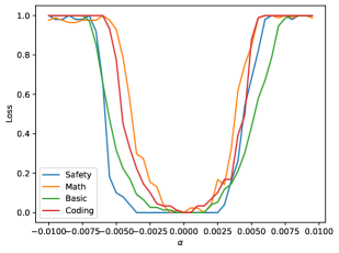
This map basically summarizes the main lines of the paper. The four curves of safety, math, basic, coding are close to 0 in the centre area for a long time, indicating that the model is almost “no drop” within the perturbation of this parameter; it can be quickly lifted to close to 1 once it continues to go out, meaning that the model-related capabilities are significantly degraded.

That's what the paper says. basinNot the smooth, round, and constantly changing bowl curves in the traditional small models, but a broad zone of stability. The author's instinct is that pre-training has pushed the model into a sufficiently large high-level stabilization subspace where small-scale moves are made, and most benchmarks are not going to break right away.

Another observation is that this type of basin is not “prevent”, but will emerge as the size of the model grows. Qwen:

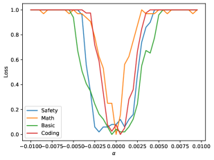
This is more like our familiar little model Landscape: The center has a low valley, but the plateau is narrow, and the four curves are more like a continuously constricted V-shaped valley than a vast and stable basin.

And then look at 32B:

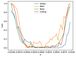
The landscape is very different. While it does not require full symmetry of the left and left, the low-damaged area in the middle is significantly wider and the model can maintain its original capacity in a wider parameter neighbourhood. One of the core observations of the paper was:The bigger the model, the bigger the basin, the more obvious and the wider it is.

This explains a common empirical phenomenon: large models are usually more “resisting” than small ones. The “resistance” here is not that it is fine, but that it is updated in most random directions and within a certain range, and it is not easy to sacrifice its capacity immediately.

Basic Basin and Capitalism Basin: What's changed for pre-training and alignment?

If we continue to follow the above figure, the paper gives an inspiring statement:Pre-training first creates the Basic Basin, then then engraves the carving inside.

The so-called basic basin is a stable area where the language that is the most basic of the models is understood, continued and dialogue. Once the model arrives through extensive pre-training, it has the minimum capability to work as a language model. The subsequent instructions were aligned, secure alignment, mathematical fine-tuning, code fine-tuning, not to transfer the model to another completely unrelated location, but more like building further narrow, more specialized sub-basins in some directions within the larger basin.

So many things are logical:

• If a certain ability corresponds to a large base, then the model is less likely to forget it when it is fine-tuned.
• If a certain capacity is narrow, then a slight improvement in the direction of the capacity may be a first-time disruption.
• The size of the base of the different model families varies, so the same data and hyperparameters can create completely different side effects in different base models.

It also reminds us not to interpret the language as "covering a thin skin with pre-training." More appropriately, alignment is re-formed in the existing landscape. Some of the plastics are sufficiently large, so the new capacity is wide enough; others are not stable enough, so once SFT continues, the most vulnerable substructures will be wiped out.

World-Case and SFT-Case: Why normal fine fine fine fine fine fine fine-tuning but can destroy a few steps

If you look at most-case, you can easily draw an overly optimistic conclusion: since most directions are safe, why is there a reality of “ten data fine-tuning one model”? The answer is... worst-case direction。

First-case landscape:

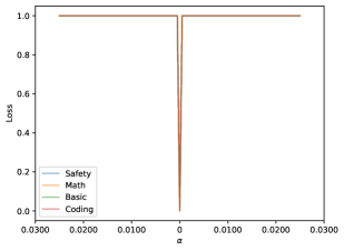
This picture is almost like a needle. In addition to the extremely narrow central areas, the four capacity curves have almost instantaneously reached the high level of the loss. The conclusions it conveys are very straightforward:While most directions are good, some extremely bad directions do exist in parameter space, and the model quickly loses almost all its capabilities as long as there is a slight deviation.

This provides a geometric explanation for “the high level of lethality of the small number of opposing data”. The counter-division is not going slowly in a random direction, but in the most negative direction. It is not about building up a large volume of updates, but about finding the export that is most likely to undermine existing capabilities.

The paper further drew the SFT direction. The author divides it into three scenarios: benign, normal and adversarial. In the first version of the text we keep the first two, because the original is basically a reconnect with the world-case.

See first, benign SFT, which is a finer finer and more moderate in the direction of the original training distribution:

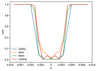
This curve remains very much like most-casebasin: the meso-stabilized zone is wide enough to indicate that the fine-tune direction is at a high altitude in the original large basin. The paper uses official versions of Qwen2.5-7B-1M to construct this direction, which you can visualize as "continue to follow the direction that the bottom model is familiar with."

And then look at the normal SFT, which is a regular downstream fine tune with clear distribution differences but not malicious data:

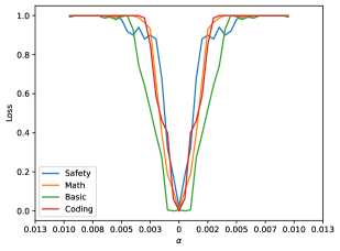
The basin became significantly narrower. It's not as exaggerating as much as the world-case, but it's no longer as relaxed as beign SFT. This means:Normal fine-tuning is still within the controlable range, but its safety residual is much smaller than most-case. As long as data distribution is more volatile, learning rates more radical and training steps longer, it is more likely that capacity will be reduced.

So, a more precise understanding is that the SFT is not in a non-black-and-black-coated division of “security” and “danger”, but rather in a continuum. The closer the training distribution, the closer the fine-tune to the original model, the closer the moste-case; the closer the deviant, the more the target is drawn, the closer the world-case.

Prompt Attack looks like Fine-Tune Attack

The original text concludes with a question: why not change the parameters, optimize the input, and also cause similar damage and fine-tuning?

The difference between the two is not as large as it appears from the first layer of activation. Set embedding $\boldsymbol{W}$, the input is $\boldsymbol{x}$。

If we disturb parameters, the first level of output becomes:

$$ (\boldsymbol{W} + \Delta \boldsymbol{W})\boldsymbol{x} = \boldsymbol{W}\boldsymbol{x} + \Delta \boldsymbol{W}\boldsymbol{x} $$

If we disturb the input, the first level of output becomes:

$$ \boldsymbol{W}(\boldsymbol{x} + \Delta \boldsymbol{x}) = \boldsymbol{W}\boldsymbol{x} + \boldsymbol{W}\Delta \boldsymbol{x} $$

So the question turns to: can you find a input disturbance? $\Delta \boldsymbol{x}$♪ That makes ♪

$$ \boldsymbol{W}\Delta \boldsymbol{x} = \Delta \boldsymbol{W}\boldsymbol{x} $$

So long as this can be done, the effects of the two attacks are the same in the first layer of activity space. The paper quoted the view that many LLM layers of embedding are now sufficiently “full” in the column space, so that the equivalent is geometrically achievable. The blogger adds:Prompt optimation can be considered a projection of parameter attack in input space.

This certainly does not mean that “all jailbreaks are worth a fine-tuning exercise”, but it explains why they often display similar vulnerabilities: They're all trying to get the model out of the stable basin, except one in the parameter space and the other in the input space for equivalent disturbances.

Basin's theoretical meaning: Clipper-Pearson, rannamozed moving and down the power line

Here, basin is still an empirical observation. The paper went further: it tried to turn this geometry into a measurable and probative object.

First, the author defined a much more soft one. $\sigma$-Basin. Intuitively, if the model parameters are added to the standard deviation $\sigma$ The Goss noise, the model's expectations are almost constant, which means it has a size. $\sigma$ BASIN:

$$ J_{f,\mathcal{D}}(\boldsymbol{\theta}) - \mathbb{E}{\boldsymbol{\epsilon} \sim \mathcal{N}(0, \sigma^2 \boldsymbol{I})}[J{f,\mathcal{D}}(\boldsymbol{\theta}+\boldsymbol{\epsilon})] \leq \varepsilon $$

The advantage of this definition is that it allows us to turn the “basin size” into a statistical object. Then there are two levels of theory.

The first level, the Clipper-Pearson base points down the directional scale.

The author will test in a large number of random directions: how many directions remain within the given radius. Because it is essentially a two-scale distribution success estimate, the Clopper-Pearson can give a strict confidence interval. So the phrase "most directions seem safe" is not just a visual image, but a "believing level." $1-\gamma$ At least... $p_{\text{lower}}$ The ratio is in the base condition.

The second layer, the ranmomid smoothing turned the base size into a sub-performance line.

The anticipatory sense given was that smoother benchmark changes would become more stable in relation to parameters once they were smoothed. Corresponds, the model is from $oldsymbol {\theta}0$ 走到 $\boldsymbol{\theta}After that, the performance drop can be restrained by the size of the base:

$$ \mathbb{E}{\boldsymbol{\epsilon}}[J(\boldsymbol{\theta}{\text{sft}}+\boldsymbol{\epsilon})] \ge \Phi\left( \Phi^{-1}(\mathbb{E}_{\boldsymbol{\epsilon}}[J(\boldsymbol{\theta}0+\boldsymbol{\epsilon})])- \frac{\lVert \boldsymbol{\theta}{\text{sft}}-\boldsymbol{\theta}_0 \rVert_2}{\sigma} \right) $$

No need to remember the formula.The same fine-tuned distance.$\sigma$ The bigger the base, the wider the performance is.

But restraint is also needed here. The paper itself acknowledges that the theoretically guaranteed “certified region” is usually much smaller than the empirically observed basin. In other words, the theoretical certificate is a conservative sub-level, not a “model that must be broken as long as it comes out of the theoretical safety zone”. Many of the conventional SFTs in reality still fall into experience, but are not fully covered by strong certificates.

Finally, emphasis is placed on border conditions: the basin discussed here is based mainly on the production of benchmark. If you switch to "likewood-based evaluation, loss landscape" you tend to re-slip the curve. This does not overturn the Basin perspective, but reminds us that the landscape you see is always about the way you choose to assess it.

Basin can be inspired by the initiative: GO optimizer

If basin means "more difficult to forget and less difficult to get hit in the worst direction," then there is naturally a question of follow-up:Can the basin be expanded?

The paper gives a directional answer that can be tried. They introduced a Gaussian-augmented Optimizer (GO optimizer), which was trained to optimize not only single-point parameters but rather expectations in the adjacent area of the parameters:

$$ L_{\text{train}}(\boldsymbol{x}, \boldsymbol{\theta}) = -\mathbb{E}_{\boldsymbol{\epsilon} \sim \mathcal{N}(0, \sigma^2\boldsymbol{I})}[\log p(\boldsymbol{x} \mid \boldsymbol{\theta}+\boldsymbol{\epsilon})] $$

Intuitively, it is a small disturbance in the adaptation of the model to the parameter neighbourhood, thus optimizing single points into a relatively good decomposition of a neighbourhood.

Here's a map of GPT2-127M, compared to Landscape, which was pretrained on OpenWebText, with the red line GO, the green line AdamW:

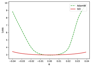
As you can see in the figure, the Go curve is evener and wider, which means that it learns not a sharp point, but a more stable region.

This wider basin also shows the benefits in the subsequent fine-tuning. The following is a comparison of the performance of the subsequent training on Alpaca: the left axis is NLL for the old capability OpenWebText and the right axis is NLL for the new capability Alpaca.

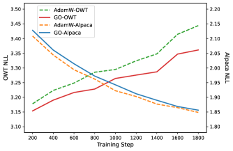
Not absolute values, but trends: the model that GO pre-trained is not learning much slower when new assignments are being taught, but the old capacity is falling even less. This corresponds to the main thesis line:If you're going to be a little broad in pre-training, then the chances of a catastrophic memory of SFT follow-up are even lower.

Of course, this part is far from being an industrial conclusion. The paper was validated only on smaller models and was more like a clear research inspiration than a direct recipe to all production systems. But it did bring the matter of “reduce the forget”, from the question of post-training techniques to the question of pre-training geometry.

To bind the whole article in three words, it's probably:

• The parameter space of the large model is not even and pre-training will shape a huge basin.
• Alignment and conventional fine-tuning are usually shaped inside the base, while anti-data can lead the model in the worst direction.
• If the model is to be more stable, the focus is not only “a little less than a parameter”, but also “can it be possible to make the space around the model more securely mobile”.

Supplement: Second reflections on the dynamics of the public valley to multitasking

The following section is an additional one. I quote and respond to the blog Sun X published at 2026-03-10.Second think about the big model, Los Landscape: the dynamic depth of gaming intelligence and universal intelligenceI'm sorry. The following are mainly re-transposing and extending the blog ' s views, not representing the direct claims of the original author; the discussion of multi-mission dynamics, the Hessian neighbourhood size and the data mix is more appropriate as an inspiration than as a conclusion that the original paper has strictly proved.

Is the public valley floor equal to universal intelligence?

The most valuable thing about this blog is that it does not directly equate "sharing the bottom of the valley on the proximity parameters of different tasks" with "models have found some sort of pure universal intelligence kernel." Bloggers are very vigilant about this optimistic interpretation: If the public valley really means that there is a “pure public knowledge base” that can be independently obtained from multi-mission training, then, by this logic, we would seem to need only a few pre-trainings, leaving the remaining tasks to be activated. But this is not the case, and the large models of good performance almost all rely on large-scale, heterogeneity, cross-cutting data mix pre-training.

Linking this suspicion to the Basin narrative, I prefer to interpret the "public valley floor" as one.A stable compromise area under multi-mandate constraintsInstead of a single mandate, there is ample evidence that everything can be taken from it. The original paper showed us that different capabilities can be maintained at the same time in the nearest region at the low of benchmark loss; but it suggests at best that the model found a set of shared signs and robust parameterizations in the region, which is not sufficient to introduce “a purely public knowledge that is not related to multitasking language material”.

If we continue to follow this perspective, it is easier to understand why the pre-training phase needs to be as rich, heterodox and broad as possible: not because the model has a purely generic knowledge core before being inserted into another mission; but becauseA sufficient number of tasks and data distributions are part of the plasticization that makes it more likely to form a stable public area.。

Why would multitask reduce the exploration dimension of search parameters space?

The instinct of blogs is that multi-mission training is an important function, not only of learning a few more things about models, but also of learning about them.Reduce the dimension of exploration in search parameters spaceI'm sorry. This is a very natural statement, if it is taken from the geometry of the parametric model.

For a large, highly parametric model, single-mission training is usually not just one of the best, but a whole low-loss stream. Intuitively, the model has a large amount of parameters that can compensate for each other: You change the parameters in some directions, the loss of task A is almost unchanged, so the optimizer can "show" in this wide flat area. Geometrically, these directions are the cutting space for low-floating single-tasks and the freedom that is most easily wasted during model searches.

Once mission B, mission C folds in, things change. Each mission defines its own low-loss flow, and multi-task learning seeks the intersection of these streams. Once multiple high-dimensional low-intensity areas are turned over, the direction that can be preserved at the same time will be significantly reduced; many of the “free-sliding” that was previously harmless only for mission A, which appears to be steeply upward, and they will be erased directly by new gradient signals.

So I'll read "reduce the dimension of exploration" as follows:Reducing the degree of ineffectiveness rather than turning the optimisation problem magically into a low-dimensional linear problem. From the point of view of optimising dynamics, search no longer occurs on a vast plain that can run around, but more like entering a narrower and more restricted public passage.

The mathematical instinct of the curve, the Hessian and the optimal neighbourhood size.

The most critical mathematical instinct in the blog comes from the inclusion of the total loss of multiple tasks as a weight:

$$ \mathcal L(\theta) = \sum_{i=1}^m \alpha_i \mathcal L_i(\theta) $$

If it's the best part of the world, $\theta^*$ The next step is to do a second-order approximation of individual tasks.

$$ \mathcal L_i(\theta) \approx \mathcal L_i(\theta^) + \frac{1}{2}(\theta-\theta^)^\top H_i(\theta-\theta^*) $$

Here. $H_i$ It's the first. $i$ Hessian, a mission, it's painted the loss local curvature in all directions. So, after supersing the multi-mission losses together, the model is allowed to remain "no more than error" $\epsilon$"the best neighbourhood, which can be written as:

$$ \delta(\epsilon)=\left{\theta:(\theta-\theta^)^\top\left(\sum_i \alpha_i H_i\right)(\theta-\theta^)\le 2\epsilon\right} $$

This collection can be seen as a super ellipse decided by the General Hessian. If you remember

$$ H_{\text{total}} = \sum_i \alpha_i H_i = Q\Lambda Q^\top $$

of which $\Lambda = \mathrm{diag}(\lambda_1,\dots,\lambda_k)$ It's a characteristic value in the curvature space, so in the main axis coordinates, the upper bounds become

$$ \sum_{j=1}^k \lambda_j z_j^2 \le 2\epsilon $$

So the radius of each main axis is...

$$ r_j = \sqrt{\frac{2\epsilon}{\lambda_j}} $$

That is, the larger the characteristic value in a given direction, the smaller the radius of parameters that can be tolerated in this direction. Further, in the chorus, the size of the super ellipse is satisfied.

$$ V(\epsilon) \propto \prod_{j=1}^k \sqrt{\frac{2\epsilon}{\lambda_j}} = \frac{(2\epsilon)^{k/2}}{\sqrt{\prod_{j=1}^k \lambda_j}} $$

This is the mathematical intuitive source of blogs that say "multitasks will compress the best neighbourhood size": when Hessian is almost independent and not exactly in the same direction as he is bound by multiple tasks, he is not the only one who is the best in the world to be able to use his own tools.$H_{\text{total}}$ The active feature values will be raised as a whole and many of the flat directions that were close to zero will be activated by additional constraints. As a result, the viable neighbourhood that meets the same tolerance for error is significantly reduced.

Of course, it must be clear here: It's a...Understand the math instincts of blogging., not the complete conclusion that has been rigorously proved in the present paper. The practical training is not only about the near-defunct of the local second stage, but also about the complexity of non-compression, re-alignment of parameters, and non-exchangeability of different tasks. So it's more like a approximation that helps us understand why multiple missions compress ineffective freedom than a theory that can be mechanically applied.

Is a multi-module considered a stronger multi-task?

My judgment is:It can, and usually can, be seen as a more binding, more isomeric multitask. For VLM or more generic multi-modular models, a simple joint goal can be written as:

$$ \mathcal L_{\text{total}} = \alpha \mathcal L_{\text{text}} + \beta \mathcal L_{\text{vision}} + \gamma \mathcal L_{\text{align}} $$

These include both text-modeling losses and visual modelling losses, as well as cross-modular alignment losses. These constraints are much more isomeric than the multiple tasks in the text: the text is a discrete symbol structure, the visual is a continuous, dense signal, and cross-modular alignment requires that both are mapd in shared semantic spaces.

From the Hessian perspective, the multimodules are more binding than “more tasks”, but rather because the different mosaics are cutting more closely to the cross-section of parameter space. Some direction is almost zero-costed in pure text missions, and in visual missions it may immediately become high curvature; while some of the redundant direction of visuality may be re-locked by language alignment losses. So the overall Hessian active feature values are more likely to be raised as a whole, with the original large numbers of nulk-space and near-zero curvatures being cut, and the optimal neighbourhood size to meet the same error threshold is more likely to continue to contract.

But I'd like to add a conservative sentence here:Smaller neighbourhoods do not automatically mean that training is easier. Multiple models bring not only greater restraint, but also greater optimization of instability, model conflicts and training rigidity. It is true that it may be more conducive to the development of cross-model public concepts, but it is equally likely to drag models into more optimised states if the loss matching, sampling sequence, architecture interfaces and alignment of targets are sufficiently rational.

The value of isomer feedback may lie not only in providing more information to the model but also in remodeling the los landscape, the ineffective, speculative and cheating exploration channels in compressed policy space. If this judgement is generally true, the future is better in terms of data mixing data by knowledge coverage or geometrically combined data — that is, which tasks, which models, which feedback should come together to move the model more effectively to the public flat valley floor, which is difficult to cheat and which is migratory.

References

• Huanran Chen et al., Unveiling the Basin-Like Loss Landscape in Large Language Models. arXiv Summary Page
• Sun X, Second think about the big model, Los Landscape: the dynamic depth of gaming intelligence and universal intelligence. Original Link （2026-03-10）